Chapter 6. NGS Application for Genomics
The Fundamental Question: Why Not Always Sequence Everything?
If sequencing technology can read all 3.2 billion base pairs of the human genome, why would we choose to sequence only part of it? It’s a bit like asking: if you’re looking for a lost key in your house, why not search every room, every drawer, every pocket? The answer is simple: time, cost, and practicality.
In genomics, we face a similar trade-off. You can sequence:
- The whole genome - all 3.2 billion bases, every gene and every space between genes
- Just the exome - only the ~30-50 million bases that code for proteins (about 1-2% of the genome)
The choice between these approaches has shaped how we discover disease genes, diagnose patients, and conduct research. Let’s understand what each approach offers and when to use which one.
Understanding the Exome: Where Most Disease Variants Hide
Before we compare WGS and WES, we need to understand what the exome is and why it’s special.
Your genome contains about 20,000 protein-coding genes. But genes aren’t continuous stretches of DNA. Instead, each gene is split into:
- Exons: the parts that code for proteins (typically 50-200 bases each)
- Introns: the non-coding parts between exons (often thousands of bases long)
When cells make proteins, they transcribe the entire gene into RNA, then cut out the introns and splice the exons together. The final messenger RNA (mRNA) contains only exonic sequence, which is then translated into protein.
The collection of all exons in the genome is called the exome. It makes up only 1-2% of your total DNA about 30-50 million base pairs out of 3.2 billion. But here’s why it’s important:
About 85% of known disease-causing mutations occur in exons.
Why? Because exons directly code for proteins. A single base change in an exon can swap one amino acid for another (missense), create a premature stop signal (nonsense), or shift the reading frame (frameshift). Any of these can break a protein’s function, potentially causing disease. Changes in introns or intergenic regions can affect gene regulation or RNA splicing, but they’re less likely to have dramatic effects.
This high concentration of disease variants in exons created an opportunity: if most pathogenic variants are in just 1-2% of the genome, we could focus our sequencing there.
Head-to-Head Comparison: WES vs WGS
Before diving into details, let’s see how these approaches compare:
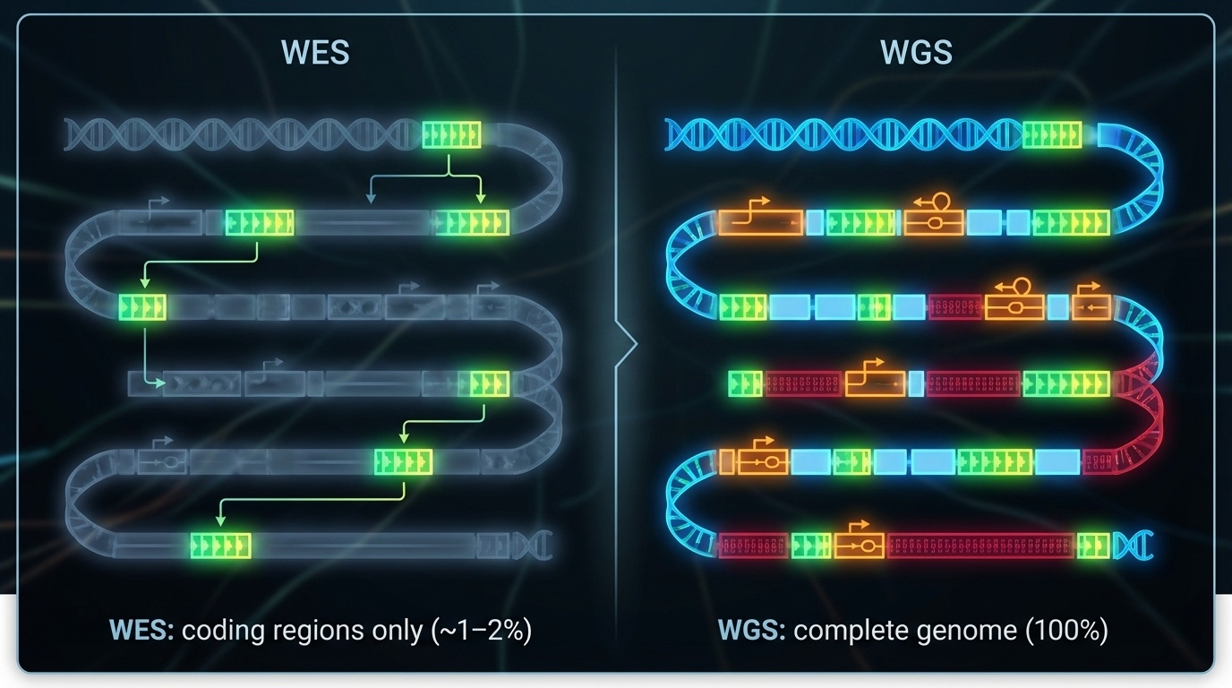
Figure 6-1. WES vs WGS: What Do You See? WES targets only the coding regions (exons), capturing about 1-2% of the genome where most disease-causing variants reside. WGS sequences the entire genome, including exons, introns, and regulatory regions, providing complete coverage but at higher cost and complexity.
| Feature | Whole-Exome Sequencing (WES) | Whole-Genome Sequencing (WGS) |
|---|---|---|
| Coverage | ~1-2% of genome (exons only) | 100% of genome |
| Target size | 30-50 million bases | 3.2 billion bases |
| Data per sample | ~6 GB | ~90-100 GB |
| Cost (2024) | ~$400-500 | ~$600-1,000 |
| Typical depth | 100-150X | 30-40X |
| SNVs/indels in exons | ✓ Excellent | ✓ Excellent |
| Structural variants | ✗ Mostly missed | ✓ Detected |
| Non-coding variants | ✗ Missed | ✓ Detected |
| Regulatory regions | ✗ Missed | ✓ Detected |
| Repeat expansions | ✗ Missed | ✓ Detected (especially with long reads) |
| Analysis complexity | Lower fewer variants | Higher millions of variants |
| Interpretation | Easier focus on coding | Harder non-coding interpretation uncertain |
| Diagnostic yield (rare disease) | 25-50% | 30-55% (slightly higher) |
| Best for | Known coding disorders, cost-sensitive studies | Complex cases, structural variants, discovery |
Whole-Exome Sequencing (WES): The Focused Approach
How It Works
WES doesn’t actually sequence only exons that would be technically challenging. Instead, it uses a clever trick called target capture or enrichment:
- Extract DNA and break it into fragments (just like WGS)
- Add special “bait” molecules short DNA sequences complementary to exons, labeled with biotin
- These baits bind to exonic fragments through complementary base pairing
- Add streptavidin-coated magnetic beads that bind tightly to biotin
- Use a magnet to pull down the beads with captured exons attached
- Wash away non-exonic DNA (introns, intergenic regions get discarded)
- Release and sequence only the captured exonic fragments
Think of it like using a magnet to pick out just the metal pieces from a mixed pile of materials.

Figure 6-2. WES Process with Target Capture. After DNA extraction and fragmentation, biotinylated probes (baits) bind specifically to exonic sequences. Streptavidin-coated magnetic beads capture these probe-bound fragments, physically separating exons from introns and intergenic regions. This targeted enrichment concentrates sequencing effort on the protein-coding regions. Source: Microbe Notes
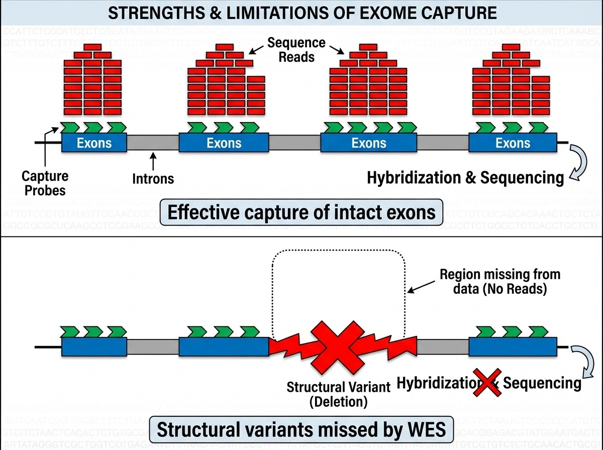
Figure 6-3. Why Target Capture Works and Why It Fails. Top: When exons are intact, capture probes bind efficiently and generate high-depth sequencing data. Bottom: Structural variants like deletions or duplications prevent probe binding, leaving these regions undetected in WES data. This fundamental limitation explains why WES misses 5-10% of pathogenic variants that WGS can detect.
Commercial capture kits from companies like Agilent SureSelect, Illumina TruSeq, and Twist Bioscience each target slightly different exon sets with varying capture efficiencies. Not all exons capture equally well regions with extreme GC content, repetitive sequences, or complex secondary structures often have coverage gaps.
The Historic Success: Miller Syndrome (2010)
WES made its breakthrough in 2010 with a paper that became a model for the approach. Researchers were studying four siblings with Miller syndrome a rare developmental disorder causing facial abnormalities. Traditional gene-hunting methods had failed.
The strategy was simple but revolutionary:
- Sequence all exons in the four affected siblings
- Look for variants they share but their healthy parents don’t have
- Focus on rare variants (not common polymorphisms)
They found variants in a gene called DHODH that none of the healthy family members carried. DHODH had never been linked to any human disease before. This discovery took months instead of years and cost thousands instead of millions.
This paper launched the WES era. Suddenly, researchers could identify disease genes for rare disorders by sequencing just a few affected individuals.
Clinical Impact of WES
WES quickly became the first-line genetic test for diagnosing rare diseases, with a diagnostic yield of 25-50% for patients with suspected genetic disorders, WES identifies the genetic cause in roughly one-third to half of cases. This is remarkable considering these patients often underwent years of inconclusive testing.
When WES works well:
- Rare Mendelian disorders (single-gene diseases)
- Diseases known to be caused by coding variants
- When you need to screen many genes at once
- When cost is a consideration
When WES comes up short:
- No variant found in known disease genes
- Patient’s disease might be caused by non-coding variants
- Structural variants might be involved (WES cannot detect large deletions, duplications, or rearrangements)
- Coverage gaps in technically challenging exons
Whole-Genome Sequencing (WGS): The Comprehensive Approach
How It Works
WGS is conceptually simpler than WES you just sequence everything:
- Extract DNA and break it into fragments
- Add adapters for sequencing
- Sequence all fragments
- Align to the reference genome
No target capture step. No enrichment. Just sequence the whole thing.

Figure 6-4. Whole-Genome Sequencing (WGS) Workflow. WGS captures all genomic regions coding exons, introns, regulatory elements, and intergenic sequences without the selective enrichment step used in WES. This comprehensive approach enables detection of all variant types. Source: Microbe Notes
The Power of Seeing Everything: Real Examples
Structural variants: A patient with developmental delay and seizures tested negative on WES. WGS revealed a large deletion removing three exons of a neurodevelopmental gene. WES missed this because target capture requires intact DNA when exons are deleted, there’s nothing for the baits to capture. WGS detected the deletion through absence of reads in that region. This happens in about 5-10% of cases where WES fails.
Regulatory variants: Some forms of beta-thalassemia (reduced hemoglobin production) are caused by mutations in the regulatory regions of the HBB gene, not in the coding sequence. These would be missed by WES but are detectable with WGS.
Deep intronic variants: While WES captures exon-intron boundaries, deep intronic variants can create new splice sites or destroy existing ones. These “cryptic splice variants” can cause disease but lie beyond WES’s reach.
Non-Coding Variants: The Frontier
WGS opens up the study of non-coding variants, which make up 98% of the genome. While most non-coding sequence is functionally neutral, some regions are critically important. Enhancers and promoters control when and where genes are expressed a mutation in an enhancer can affect a gene hundreds of thousands of bases away, causing disease without touching the gene itself.
The challenge: We’re still learning which non-coding variants matter. The human genome contains millions of non-coding variants, and distinguishing functional from neutral ones remains difficult.
The Technical Process: From Sample to Variants
Whether you’re sequencing a whole genome or just the exome, the basic workflow is similar with one key difference for WES: target capture to isolate exons. This section walks through the laboratory and computational steps that transform a blood sample into a list of genetic variants.
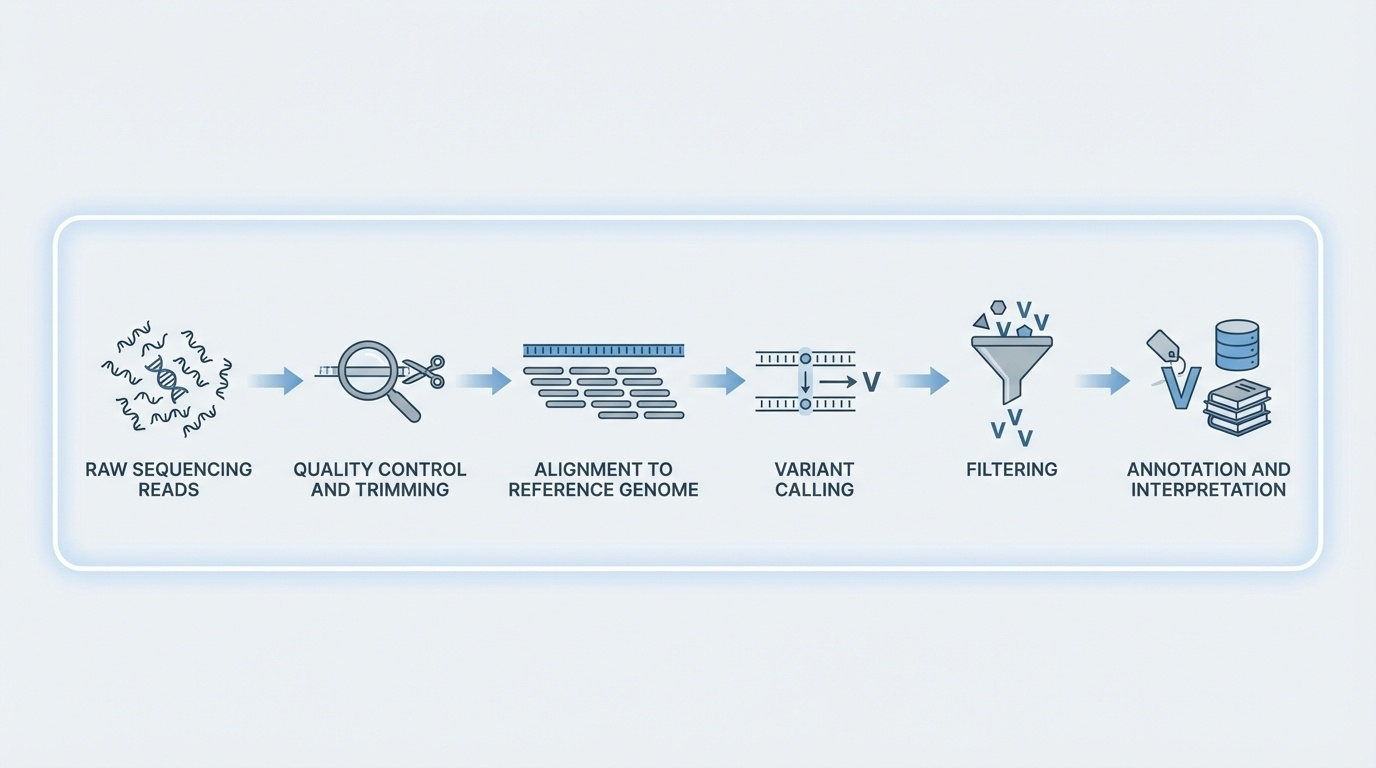
Figure 6-5. From Reads to Variants: The Computational Pipeline. After sequencing generates millions of reads, a series of computational steps transforms raw data into clinically actionable variants: quality control removes low-quality bases, alignment maps reads to the reference genome, variant calling identifies differences, filtering removes artifacts, and annotation adds biological context.
Step 1: Library Preparation
Library preparation is the process of converting your DNA sample into a form that sequencing machines can read. The workflow differs significantly between short-read platforms (Illumina) and long-read platforms (PacBio, Nanopore), each optimized for their specific sequencing chemistry.
A. Illumina Library Preparation (Short-Read Sequencing)
Illumina library prep is the most common approach for both WGS and WES, optimized for generating billions of short, highly accurate reads.
📺 Video Resource: For a detailed walkthrough of Illumina library preparation, watch this Illumina expert tutorial which covers best practices for Nextera library prep.
Overview of the Workflow:
1. DNA Extraction and Quality Control
- Input: ~1 μg for WGS, ~200-500 ng for WES
- Quality matters: degraded DNA leads to poor results
- Assessed using spectrophotometry (UV absorbance) and fluorometry
2. Fragmentation
- Why fragment? Illumina sequencers can’t read long molecules
- Methods: Sonication (ultrasound) or enzymatic digestion
- Target size: 150-500 bp fragments
- Result: DNA broken into manageable pieces for short-read sequencing
3. End Repair and Adapter Ligation
- DNA fragment ends are “ragged” after fragmentation
- Enzymes trim to create clean, blunt ends
- Adapters (short synthetic DNA sequences) are ligated to both ends:
- Provide primer binding sites
- Enable attachment to flow cell
- Include barcodes for multiplexing (mixing multiple samples)
4. PCR Amplification
- Amplify library to ~12-15 cycles
- Creates billions of copies for sequencing
- Trade-off: Introduces some bias (GC-rich/poor regions amplify differently)
5. Target Capture (WES Only!)
- This extra step distinguishes WES from WGS
- Uses biotinylated probes complementary to exons
- Magnetic beads capture probe-bound fragments
- Non-exonic DNA is washed away
- See WES section above for detailed explanation
6. Quality Control Check
- Bioanalyzer/TapeStation: verify fragment size distribution
- qPCR/fluorometry: measure library concentration
- For WES: confirm successful exon enrichment
Key Advantages: High accuracy (>99.9%), massive throughput (billions of reads), well-established protocols
Limitations: Short reads struggle with repetitive regions and structural variants
B. PacBio Library Preparation (Long-Read HiFi Sequencing)
PacBio library prep creates circular DNA templates that enable multiple reads of the same molecule for high-accuracy long reads.
📺 Video Resource: For PacBio and Nanopore library preparation workflows, watch this comparative tutorial.
Overview of the Workflow:
1. DNA Extraction and Quality Control
- Input: ~500 ng of high-molecular-weight DNA
- Critical: DNA must be high quality and intact fragmentation ruins long-read potential
- Use gentle extraction methods to preserve long molecules
2. Fragmentation (Gentle!)
- Target size: 15,000-20,000 bp (100X longer than Illumina!)
- Uses controlled shearing to maintain longer fragments
- Can skip fragmentation entirely for ultra-long molecules
3. End Repair and Hairpin Adapter Ligation
- Clean up fragment ends
- Key difference: Add hairpin adapters to create SMRTbell templates
- SMRTbell = circular DNA molecule (template loops back on itself)
- This circular structure allows the polymerase to read the same molecule multiple times
4. No PCR Amplification (Usually!)
- PacBio HiFi often sequences native DNA directly
- Skipping PCR eliminates bias and preserves DNA modifications (methylation)
- Enables detection of epigenetic marks
5. Quality Control Check
- Verify fragment length distribution (critical for long reads)
- Check SMRTbell template integrity
- Quantify library concentration
The HiFi Advantage: The polymerase circles the SMRTbell template 10-20 times, reading the same DNA sequence repeatedly. A consensus is computed from these multiple passes, achieving >99.9% accuracy despite long read lengths.
Key Advantages: Long reads (10-20 kb), high accuracy, no PCR bias, detects DNA modifications
Limitations: Lower throughput than Illumina, higher cost per base
C. Oxford Nanopore Library Preparation (Ultra-Long Read Sequencing)
Nanopore library prep is the simplest and fastest, enabling ultra-long reads and even portable sequencing.
📺 Video Resource: See the comparative tutorial mentioned above for Nanopore workflows.
Overview of the Workflow:
1. DNA Extraction and Quality Control
- Input: Variable (can work with very small amounts)
- Goal: Extract ultra-high-molecular-weight DNA
- Some protocols achieve >100 kb, even >1 Mb intact molecules
2. Minimal or No Fragmentation
- Nanopore can sequence native, unfragmented DNA
- Longer molecules = longer reads
- Some protocols skip fragmentation entirely
3. Adapter Ligation
- Two approaches:
- Ligation-based: Adapters ligated to DNA ends (more accurate)
- Transposase-based (Rapid Kit): Faster prep, slight bias in AT-rich regions
- Adapters contain motor proteins that feed DNA through nanopores
4. No PCR Amplification (PCR-Free)
- Nanopore sequences native DNA directly
- Preserves all biological information including base modifications
- Fastest library prep among all platforms (~10 minutes possible with Rapid Kit)
5. Minimal Quality Control
- Quick concentration check
- Ready to load on sequencer
The Nanopore Advantage: Simplest library prep, real-time sequencing (watch data generation live), ultra-long reads (>100 kb, sometimes >1 Mb), portable devices (MinION is USB-sized).
Key Advantages: Ultra-long reads, fastest library prep, portable sequencing, real-time results, native DNA sequencing
Limitations: Higher per-base error rate than Illumina/PacBio (though improving rapidly), lower throughput per run
Comparison: Which Platform for Which Application?
| Feature | Illumina | PacBio HiFi | Oxford Nanopore |
|---|---|---|---|
| Library Prep Time | 4-8 hours | 3-6 hours | 10 min - 2 hours |
| Read Length | 150-300 bp | 10-20 kb | 10-100+ kb |
| Accuracy | >99.9% | >99.9% | 95-99% |
| PCR Amplification | Yes (usually) | No (usually) | No |
| Best For | WES, high-throughput WGS | Structural variants, phasing | Ultra-long reads, genome assembly |
| Fragmentation | Required | Controlled | Minimal/none |
| Special Feature | Target capture for WES | SMRTbell circular templates | Motor proteins, portability |
Bottom line: Choose your platform based on your scientific question:
- Need billions of cheap, accurate reads? → Illumina
- Need to resolve structural variants or phase haplotypes? → PacBio
- Need ultra-long reads or portable/rapid sequencing? → Nanopore
Step 2: Sequencing
Illumina Sequencing (Most Common for WGS and WES)
The library is loaded onto a flow cell a glass slide with millions of tiny spots where sequencing happens.
Cluster generation: Library fragments bind to oligonucleotides on the flow cell surface, then through “bridge amplification” create dense clusters of ~1,000 identical copies. Single molecules don’t produce enough signal to detect clusters amplify the signal.
Sequencing by Synthesis (SBS):
- All four nucleotides (A, C, G, T), each with a different fluorescent dye, are added with DNA polymerase
- Polymerase adds one base to each growing strand (these are reversible terminators that block further addition)
- A camera records which color (and therefore which base) was added at each cluster
- The fluorescent tag and terminator are chemically removed
- Repeat for 150-300 cycles
This produces millions of short reads simultaneously typically 2×150 bp (paired-end sequencing, reading both ends of each fragment).
Typical output:
- WES: ~50-100 million reads (~6-10 GB of data)
- WGS: ~1 billion reads (~90-100 GB of data)
PacBio Revio Sequencing (For WGS, Especially Structural Variants)
PacBio uses SMRT Cells containing 25 million tiny wells called zero-mode waveguides (ZMWs). Each well holds a single DNA polymerase molecule.
Single-Molecule Real-Time (SMRT) sequencing:
- A single SMRTbell template (circular DNA) is loaded into each ZMW
- As the polymerase incorporates bases, it flashes brief pulses of light
- The polymerase circles around the template multiple times, reading the same sequence repeatedly
- HiFi reads: By reading the same molecule 10-20 times and taking a consensus, PacBio achieves >99.9% accuracy
Read lengths: 15,000-20,000 bp average, with some exceeding 100,000 bp. These long, accurate reads can span entire genes, resolve structural variants, phase variants, and sequence through repetitive regions.
Oxford Nanopore Sequencing (For Ultra-Long Reads)
Nanopore sequencing threads DNA through protein pores in a membrane. As bases pass through, they disrupt an electrical current in characteristic ways, enabling ultra-long reads (>100,000 bp, sometimes >1 million bp), real-time results, and portable devices like the USB-sized MinION.
Step 3: Variant Calling - From Reads to Biological Meaning
After sequencing, you have millions or billions of reads. Now comes the computational challenge: figuring out what your genome looks like and how it differs from the reference.
3.1 Quality Control of Raw Reads
Each base call comes with a quality score (Q score):
- Q20 = 99% accuracy (1 error per 100 bases)
- Q30 = 99.9% accuracy (1 error per 1,000 bases)
- Q40 = 99.99% accuracy (1 error per 10,000 bases)
FastQC checks per-base quality, sequence duplication levels, adapter contamination, and GC content distribution. Low-quality bases (typically at read ends) and adapter sequences are trimmed.
3.2 Alignment to Reference Genome
Your reads need to be mapped back to their original genomic positions.
Alignment tools:
- BWA (Burrows-Wheeler Aligner): Standard for Illumina short reads
- Minimap2: Designed for long reads (PacBio, Nanopore)
The aligner compares each read to the reference genome (e.g., GRCh38 or T2T-CHM13), finds the best-matching location, and produces a BAM file (Binary Alignment Map).
Challenges: Repetitive regions create ambiguity for short reads. Structural variants can cause incorrect alignment or prevent alignment entirely.
3.3 Removing PCR Duplicates
PCR created many identical copies of some original DNA molecules. Tools like Picard MarkDuplicates identify and mark duplicates based on identical mapping positions and sequences. Duplicates inflate coverage artificially and can bias variant calling.
3.4 Variant Detection
Sophisticated software tools use statistical models to distinguish real variants from sequencing errors.
Popular tools:
- GATK (Genome Analysis Toolkit): The gold standard from the Broad Institute
- FreeBayes: Bayesian variant caller
- DeepVariant: Uses deep learning/AI from Google
How it works: For each genome position, the variant caller stacks up all covering reads, counts bases, calculates the likelihood of a real variant versus sequencing error, considers quality scores, checks depth (20-30+ reads provide confidence), and applies statistical filters.
Example:
- Position chr1:12345 in reference: G
- Your sample: 28 reads show A (all Q30+), 2 reads show G (Q15, Q20)
- Conclusion: Likely a real homozygous SNP (A/A instead of G/G)
Output: A VCF file (Variant Call Format) listing all detected variants with position, reference/alternate bases, quality score, genotype, and read depth.
3.5 Filtering Variants
Initial variant calls contain false positives. Filtering removes artifacts based on:
- Minimum depth (≥10-20 reads)
- Quality threshold (≥20 or ≥30)
- Strand bias (if all supporting reads come from one strand, likely an artifact)
- Allele balance (for heterozygous variants, expect ~50% of reads showing each allele)
Result: A high-confidence variant set thousands to millions of variants depending on WGS versus WES.
3.6 Variant Annotation
Annotation tools (VEP, ANNOVAR, SnpEff) add biological context:
Genomic location: Is this in a gene? Which one? In an exon, intron, or intergenic region?
Functional impact:
- Synonymous: Changes DNA but not amino acid
- Missense: Changes amino acid
- Nonsense: Creates a stop codon
- Frameshift: Insertion or deletion shifts the reading frame
- Splice site: Affects exon joining
Population frequency: How common is this in databases like gnomAD? Common variants (>1%) are usually benign.
Clinical significance: Is it in ClinVar? What’s the classification (pathogenic, benign, VUS)?
Prediction scores: CADD, REVEL scores indicate likely deleteriousness and pathogenicity.
Output: An annotated VCF file, often converted to a spreadsheet for easier interpretation.
Putting It All Together: A Complete Workflow
Day 1-3: DNA extraction and library preparation (WES includes exome capture)
Day 4-5: Sequencing on NovaSeq 6000, generating ~80 million read pairs for WES
Day 6-7: Bioinformatics QC, alignment, duplicate marking, variant calling and filtering
Day 8-10: Interpretation filter for rare variants, focus on genes related to symptoms, prioritize high-impact variants, check ClinVar, validate with Sanger sequencing
Result: Genetic diagnosis made in ~10 days, compared to months or years with older approaches.
The Clinical Decision Tree: Which Test to Order?
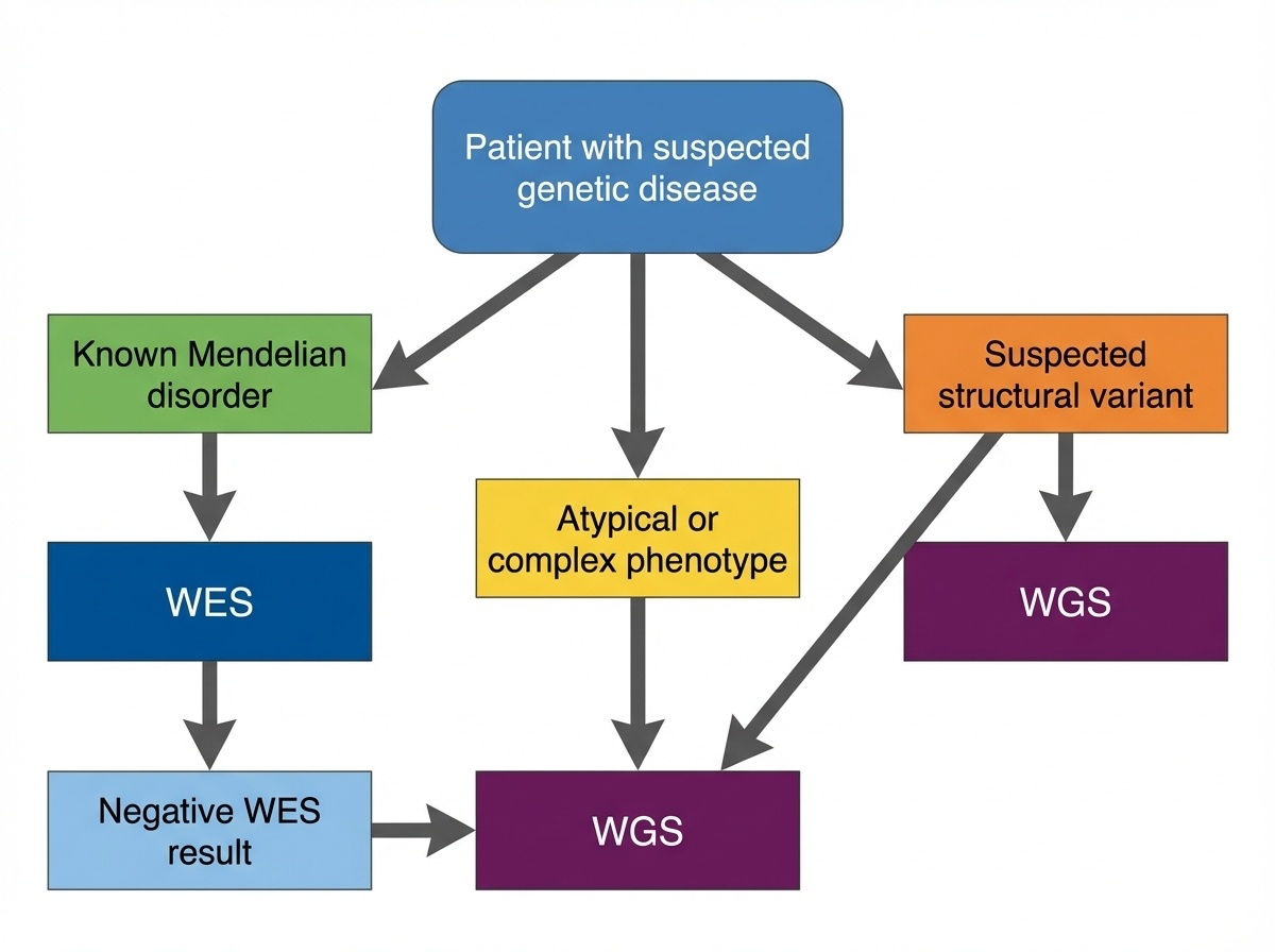
Figure 6-6. Clinical Decision Tree: WES or WGS? This flowchart guides clinical decision-making for genetic testing. Start with WES for suspected Mendelian disorders with known coding variants. Move to WGS when WES is negative, structural variants are suspected, or the phenotype is complex or atypical.
Start with WES if:
- The patient has features of a known Mendelian disorder where most causative variants are in coding regions
- You need to screen many genes simultaneously (e.g., hearing loss can involve >100 genes)
- Cost matters for large studies or resource-limited settings
- The phenotype suggests a coding variant like loss of protein function
Move to WGS if:
- WES was negative but you still suspect a genetic cause (WGS finds answers in ~10-30% of WES-negative cases)
- You suspect a structural variant (developmental delay with dysmorphic features, multiple congenital anomalies)
- The phenotype is complex or atypical and might involve regulatory variants
- You need comprehensive screening to rule out all possible genetic causes
- You want future-proof data for reanalysis as we learn more about non-coding regions
A Real Decision-Making Case
Patient: 8-year-old boy with intellectual disability, autism, and dysmorphic facial features
Testing strategy:
- Chromosomal microarray (cheap, quick) → Normal
- WES → Several variants of uncertain significance, nothing diagnostic
- WGS → 150 kb deletion removing first 5 exons of a neurodevelopmental gene
This deletion was missed by WES (no exons to capture) and too small for microarray. WGS provided the answer after other methods failed.
The Economics and Practicalities
The Cost Trajectory
The cost gap between WES and WGS is shrinking rapidly:
| Year | WES Cost | WGS Cost | Difference |
|---|---|---|---|
| 2010 | ~$5,000 | ~$50,000 | 10X |
| 2015 | ~$1,000 | ~$5,000 | 5X |
| 2020 | ~$500 | ~$1,000 | 2X |
| 2024 | ~$400-500 | ~$600-1,000 | 1.5X |
As costs converge, the argument for WES weakens. Soon, WGS may cost the same as WES.
Storage and Computing
Storage needs:
- WES: 6 GB per sample (1,000 samples = 6 TB)
- WGS: 90 GB per sample (1,000 samples = 90 TB)
For large biobanks, this 15X difference matters. The UK Biobank sequenced 500,000 genomes at 90 GB each, that’s 45 petabytes requiring serious infrastructure.
The Analysis Bottleneck
Sequencing is fast. Interpretation is slow.
- WES: ~20,000 variants per person, mostly coding with known functional effects, analyzed in days
- WGS: 4-5 million variants per person including millions of non-coding variants with uncertain interpretation, takes weeks
As one geneticist observed: “We went from being starved for data to drowning in it.”
The Future: Is WES Becoming Obsolete?
There’s an interesting argument emerging: WES might be a transitional technology.
The “WGS Now, Interpret Exome First” Strategy
You can do WGS but initially analyze only the exonic regions getting WES-equivalent results while keeping the full dataset for later. This gives you:
- Immediate WES-level analysis (just look at exons)
- Option to expand analysis to non-coding regions if exons are negative
- Future-proofing: As we learn more about non-coding variants, reanalyze the same data
What’s Driving the Shift?
- Cost convergence: WGS approaching WES pricing
- Improved long-read sequencing: PacBio and Oxford Nanopore handle structural variants and repeats better
- Better interpretation tools: AI and machine learning helping interpret non-coding variants
- Clinical evidence: WGS diagnostic yield consistently 5-10% higher than WES
But WES Isn’t Dead Yet
WES still has advantages:
- Large population studies where storage and cost matter at scale
- Focused disease studies involving known coding variants
- Lower-income settings where every dollar counts
- High coverage needs WES provides deeper coverage of exons for the same cost
A Glimpse of the Long-Read Future
Most WGS and WES today uses short-read sequencing (Illumina), which struggles with repetitive regions, structural variants, and phasing.
Long-read sequencing (PacBio HiFi, Oxford Nanopore) is changing this with reads of 15,000-20,000 bp or >100,000 bp that can:
- Span entire genes in single reads
- Reveal structural variants directly
- Phase variants naturally
- Sequence through repetitive regions
The T2T-CHM13 genome (the first complete human genome) was built using long reads. As long-read WGS becomes more affordable, it will likely replace short-read approaches.
Summary: The Bottom Line
Whole-Exome Sequencing:
- Focused, cost-effective approach targeting disease-rich coding regions
- Ideal for known Mendelian disorders
- Misses structural and regulatory variants
- Widely used clinically but likely a transitional technology
Whole-Genome Sequencing:
- Comprehensive, unbiased approach detecting all variant types
- More expensive and complex but increasingly favored as costs decline
- The future of clinical and research sequencing
The trend is clear: We’re moving toward universal WGS. For now, both approaches have their place, and the choice depends on your question, resources, and clinical context. The key insight: WES isn’t simply a subset of WGS in practice it’s a different experimental design with distinct strengths and limitations. Understanding when to use each approach is essential for modern geneticists and clinicians.