Chapter 23. Recombination, Linkage, and Haplotype
Here’s a question you’ve probably wondered about: why do siblings look different? You and your sister both got half your DNA from your mom and half from your dad, just like everyone else. So why don’t all siblings look identical?
Part of the answer is which specific half you got. Your mom has two copies of each chromosome—one from her mother (your maternal grandmother) and one from her father (your maternal grandfather). When she makes an egg cell, she passes on one of those two copies at each chromosome. You might get mostly grandma’s versions, while your sister might get mostly grandpa’s versions. That alone creates variation.
But there’s more to the story. Your mom doesn’t pass on her mother’s chromosome exactly as she received it. During the formation of egg cells—a process called meiosis—matching chromosomes pair up and actually exchange DNA segments. It’s like shuffling a deck of cards, but with chromosomes. A piece of grandma’s chromosome gets swapped with the matching piece from grandpa’s chromosome. The result? The chromosome your mom passes to you is a mosaic—part grandma, part grandpa, mixed in new combinations.
This process is called recombination, and it’s one of nature’s most elegant mechanisms for generating diversity. Without recombination, you’d inherit entire chromosomes intact from each grandparent. With recombination, you inherit pieces from all four grandparents, shuffled into novel combinations. That’s why you might have your maternal grandfather’s nose but your maternal grandmother’s eye color, even though those traits are on the same chromosome.
Recombination is also why genetic mapping works, why GWAS can find disease genes, and why we can trace ancestry. Understanding recombination is essential for understanding modern genomics.
Two Flavors of Recombination: Cross-Over and Non-Cross-Over
When geneticists first studied recombination, they focused on cross-overs (COs)—the dramatic events where large chunks of DNA get swapped between chromosomes. Cross-overs are relatively easy to detect because they create long stretches of DNA from one grandparent where you’d expect DNA from the other.
Think of cross-overs like this: imagine two ropes, one red and one blue, lying side by side. You cut both ropes at the same position and swap the cut ends. Now you have one rope that’s red on the left and blue on the right, and another that’s blue on the left and red on the right. That’s a cross-over—a clean exchange of large DNA segments.
But in 2025, something remarkable was published. By analyzing whole-genome sequences from over 5,000 Icelandic families, it was discovered that cross-overs are just part of the story. There’s another type of recombination that’s been hiding in plain sight: non-cross-overs (NCOs), also called gene conversion (Palsson et al. 2025, Nature).
Non-cross-overs work differently. Instead of swapping large segments, a small stretch of DNA—typically just a few hundred to a few thousand base pairs—gets copied from one chromosome to the other. It’s like patching a small section of the red rope with blue thread, but leaving everything else red. The overall structure doesn’t change much, but locally, you’ve altered the sequence.
Here’s what makes NCOs fascinating: they’re far more common than cross-overs. For every cross-over that happens, there might be five or ten non-cross-overs. We just didn’t realize it before because NCOs are small and hard to detect without very high-resolution sequencing data.
Both types of recombination start the same way: with a double-strand break (DSB)—a deliberate cut in both strands of the DNA double helix. Your cells make these breaks on purpose during meiosis. It sounds dangerous (and it is if it goes wrong), but it’s a controlled process. The break is repaired using the matching chromosome as a template, and depending on how the repair proceeds, you get either a cross-over or a non-cross-over.
What the Study Revealed
The first complete human recombination map that includes both cross-overs and non-cross-overs was created. Previous maps only tracked COs, so they were missing most of the action. By sequencing entire families—parents, children, and often grandparents—it was possible to trace which DNA segments came from which grandparent and spot every place where the pattern switched (Palsson et al. 2025, Nature).
The findings are striking:
Non-cross-overs vastly outnumber cross-overs. On average, each meiosis produces about 40-60 cross-overs across all 23 chromosome pairs. But it also produces several hundred non-cross-overs. That’s an order of magnitude more events, and they’d been largely invisible until now.
Mothers and fathers recombine differently. This has been known for cross-overs—maternal meiosis produces more COs than paternal meiosis. But the study found that mothers also produce longer NCOs than fathers. A typical maternal NCO might convert 1,000-2,000 base pairs, while a paternal NCO might convert only 300-500 base pairs. Why? We don’t know yet, but it suggests that the molecular machinery works differently in eggs versus sperm.
Maternal age increases non-cross-overs. As women age, the number of NCOs in their eggs goes up, especially outside the programmed recombination hotspots. This is different from cross-overs, which don’t increase much with age. The extra NCOs might be compensatory—a way to ensure that chromosomes pair correctly even when the normal CO machinery becomes less efficient with age.
Centromeres suppress cross-overs but allow non-cross-overs. Near the centromere—the pinched region in the middle of a chromosome where spindle fibers attach during cell division—cross-overs are rare. That makes sense: a CO near the centromere could disrupt chromosome segregation and cause errors. But NCOs happen readily in these regions. They might help chromosomes recognize each other and pair correctly without the risks of a full cross-over.
These patterns tell us that recombination isn’t just random DNA shuffling. It’s carefully regulated, with different mechanisms operating in different regions and at different life stages.
How CO and NCO Form: The Molecular Dance
Let’s look at what happens at the molecular level during recombination. It starts with a double-strand break—both strands of the DNA double helix are cut. This happens on one of the two paired chromosomes, let’s say the red one.
The broken DNA end is processed to create a 3’ overhang—a single-stranded tail. This tail then “invades” the matching region on the blue chromosome. It’s like the red chromosome reaching over, finding the corresponding sequence on blue, and using it as a template.
Now the cell has a choice. How does it resolve this structure?
Path 1: Synthesis-Dependent Strand Annealing (SDSA) leads to a non-cross-over. The invading strand copies some information from the blue chromosome, then pulls back and re-anneals to its original partner. The result? A small patch of DNA has been converted from the red sequence to the blue sequence, but the chromosomes don’t swap large segments. It’s a local, short-range change.
Path 2: Double Holliday Junction (dHJ) formation leads to a cross-over. Instead of pulling back, the invading strand stays attached, and DNA synthesis extends the connection. This creates two junctions where the chromosomes are physically joined. When these junctions are resolved—cut and rejoined—you get a cross-over. Large flanking regions get swapped.
Why does the cell sometimes choose one path and sometimes the other? That’s one of the big mysteries in meiosis research. There seem to be proteins that promote one outcome versus the other, and the local chromatin context (how tightly the DNA is packaged) probably matters too.
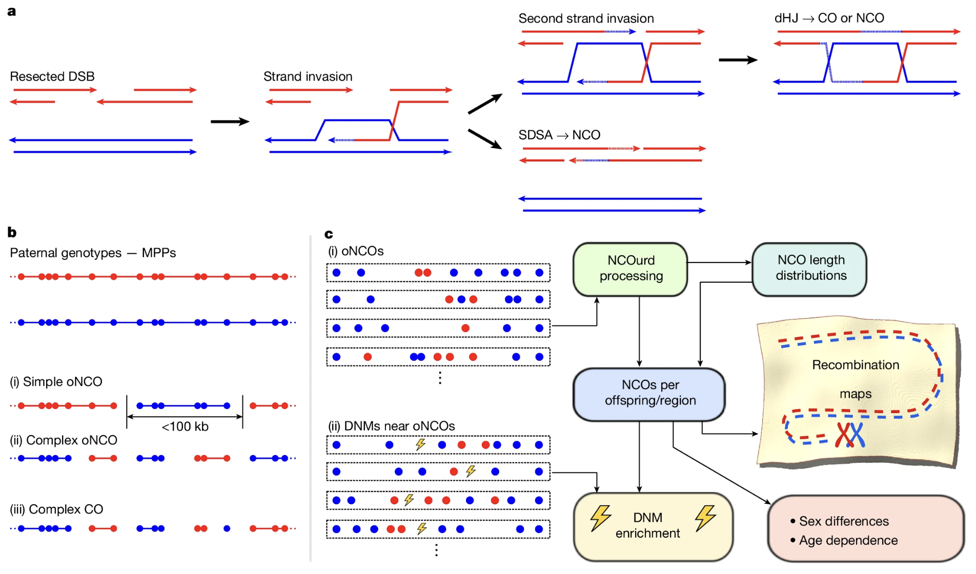
Figure: From DNA breaks to recombination maps—how the study detected and analyzed recombination events. Panel (a) illustrates the molecular mechanism of meiotic recombination. Red and blue represent the two homologous chromosomes (one from each grandparent). The process begins when a double-strand break (DSB) is deliberately made in one chromosome (red). The broken end is processed to create a single-stranded tail, which then invades the partner chromosome (blue) to search for the matching DNA sequence. From this point, two different pathways can occur. In the top pathway, a second strand also invades, forming a structure called a double Holliday junction (dHJ), which can be resolved to produce either a cross-over (CO) or a non-cross-over (NCO). In the bottom pathway, called synthesis-dependent strand annealing (SDSA), the invading strand copies a small segment of information from the blue chromosome, then pulls back and rejoins its original red partner—this always produces an NCO. Panel (b) shows how recombination events were detected in real family data. The top shows parental genotypes marked as red and blue dots (representing DNA variants from each grandparent). Below are examples of detected events: (i) a simple NCO where a short stretch switches from red to blue, (ii) a complex NCO with multiple switches in a small region, and (iii) a complex CO involving larger-scale exchanges. Panel (c) outlines the computational pipeline used to identify and characterize these events across thousands of families, ultimately producing complete recombination maps and revealing patterns like sex differences and maternal age effects. Source: Palsson, B. et al. (2025). Meiotic recombination shapes the landscape of genome variation. Nature. https://www.nature.com/articles/s41586-024-08450-5. License: CC-BY-NC-ND 4.0.
Linkage: Alleles That Travel Together
Now let’s connect recombination back to the concept of linkage we learned about in the previous section. Linkage describes the tendency of alleles located close together on the same chromosome to be inherited together.
Why does this happen? Because recombination—whether CO or NCO—is a random process with respect to position (though it’s biased toward hotspots, as we’ll see). The closer two genetic variants are, the less likely that a recombination event will occur between them. And if no recombination separates them, they “travel as a pair” from parent to child.
We quantify linkage using the recombination fraction (r). This is the probability that two loci will be separated by recombination in a single meiosis:
- r = 0 means the loci are completely linked. They’re so close together that recombination never separates them, so they always travel together.
- r = 0.5 means the loci are unlinked. They recombine half the time, which is what you’d expect for loci on different chromosomes or very far apart on the same chromosome. This is independent assortment—Mendel’s second law.
- r = 0.1 means the loci recombine 10% of the time. They’re close enough to show linkage, but far enough apart that occasional recombination separates them. This corresponds to about 10 cM of genetic distance.
The smaller the recombination rate, the stronger the linkage. Two SNPs that are only 1 kb apart might have r = 0.0001—they’re almost never separated. Two SNPs that are 10 Mb apart might have r = 0.15—they’re separated fairly often.
Linkage is why genetic mapping works. If a disease gene is located near a particular DNA marker, that marker will often be inherited along with the disease allele. By tracking which markers co-segregate with the disease in families, you can narrow down where the disease gene must be. This principle underlies linkage analysis for Mendelian diseases and, in a modified form, genome-wide association studies (GWAS) for complex traits.
The study improved our understanding of linkage in two ways. First, by including NCOs in the recombination map, it captured the full picture of how often alleles get separated. NCOs can break linkage too, even if they don’t swap large segments. Second, it showed that recombination rates vary by sex and age, which affects how strong linkage is depending on whether you’re tracing maternal or paternal transmission (Palsson et al. 2025, Nature).
Regional Differences: Not All Chromosomes Recombine Equally
If recombination were evenly distributed across the genome, genetic mapping would be simple. But it’s not. Some regions are hotspots where recombination happens frequently. Others are coldspots where it’s rare. And some regions, like centromeres, have their own special rules.
Let’s look at the patterns:
Telomeres (chromosome ends) are rich in cross-overs. When you plot CO frequency along a chromosome, you see peaks near the telomeres. This makes sense: COs near the ends don’t disrupt the chromosome’s structure much, and they help ensure proper segregation during meiosis. If chromosomes don’t have at least one CO, they might fail to separate properly, leading to aneuploidy (wrong number of chromosomes).
Centromeres (chromosome centers) suppress cross-overs but allow non-cross-overs. A CO near the centromere could interfere with how spindle fibers attach and pull chromosomes apart. So evolution has selected against COs in these regions. But NCOs still happen, and they might serve a function—perhaps helping the chromosomes recognize each other and pair up during early meiosis.
Hotspots are scattered across the genome. These are short (1-2 kb) regions where recombination—both CO and NCO—occurs much more frequently than average. Hotspots are marked by a DNA-binding protein called PRDM9, which recognizes specific sequence motifs and recruits the machinery that makes double-strand breaks. Most recombination events cluster at these hotspots.
Interestingly, hotspot locations vary between populations. A hotspot active in Europeans might be inactive in East Asians, and vice versa. This is because PRDM9 itself is highly variable—different versions recognize different DNA motifs. Over evolutionary time, hotspots can move around the genome as PRDM9 variants spread through populations.
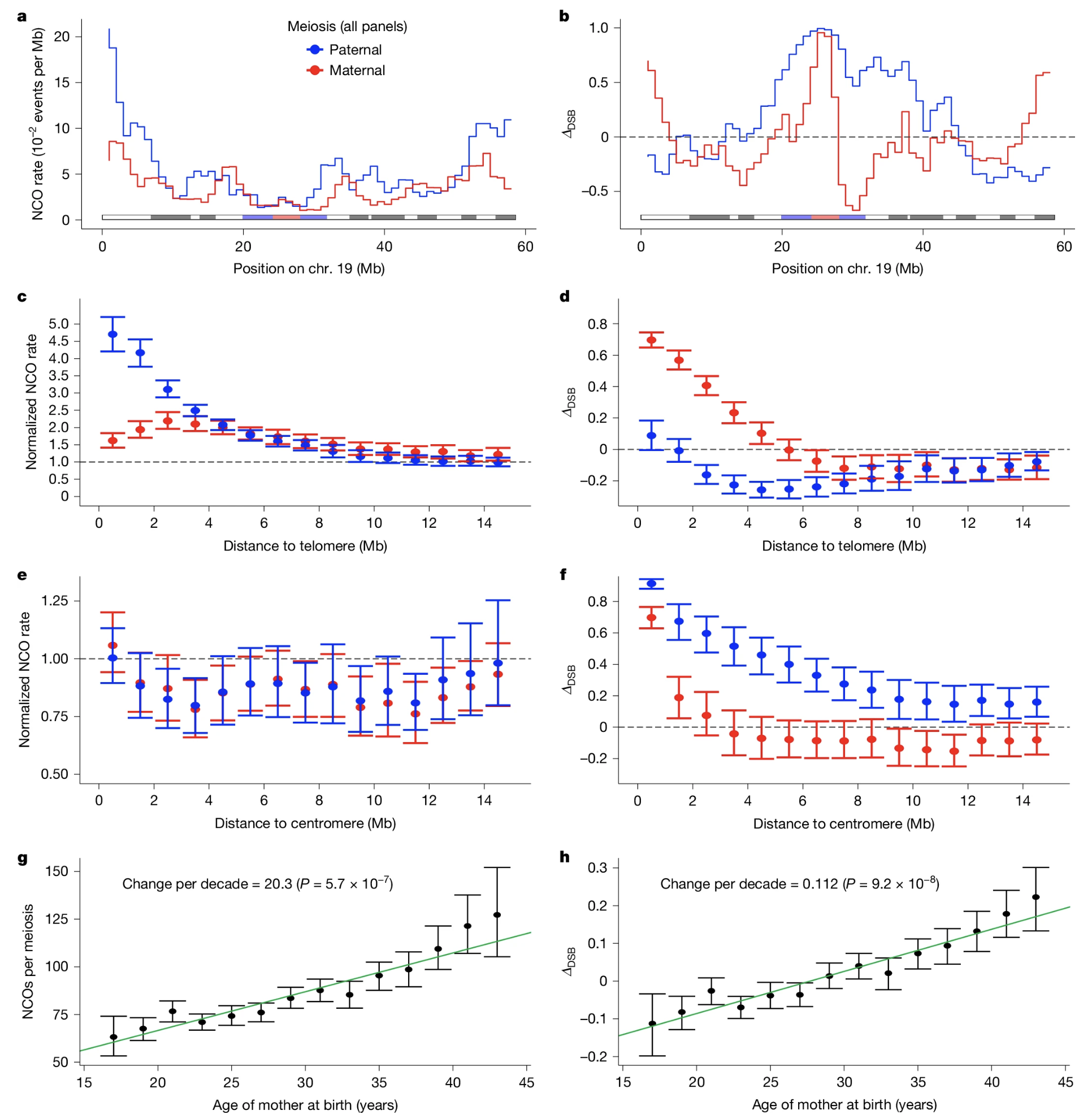
Figure: Recombination shows clear patterns: it differs between moms and dads, varies across the chromosome, and changes with maternal age. This figure uses chromosome 19 to illustrate key patterns in recombination. Panel (a) shows how frequently non-cross-overs (NCOs) occur at different positions along the chromosome. Notice that paternal NCOs (blue line) are much more frequent near the chromosome ends, while maternal NCOs (red line) show lower overall rates. The gray bar marks the centromere location. Panel (b) displays a metric called ΔcsB that indicates whether recombination events resemble cross-overs (positive values) or non-cross-overs (negative values). Maternal meiosis tends to produce more CO-like events (red line above zero), while paternal meiosis produces more NCO-like events (blue line below zero). Panels (c-d) zoom in on regions near telomeres (chromosome ends): paternal meiosis produces many more NCOs here than maternal meiosis, and this sex difference is especially pronounced. Panels (e-f) examine regions near the centromere (chromosome center): here the NCO rates are more similar between sexes, though the CO/NCO balance still differs. Panels (g-h) reveal a striking maternal age effect: as mothers get older, they produce significantly more NCOs per meiosis (about 20 additional NCOs per decade of age), and their recombination pattern shifts to become more CO-like. These findings demonstrate that recombination is tightly regulated and influenced by sex, chromosomal location, and age. Source: Palsson, B. et al. (2025). Meiotic recombination shapes the landscape of genome variation. Nature. https://www.nature.com/articles/s41586-024-08450-5. License: CC-BY-NC-ND 4.0.
The study also revealed age-related changes. As women age, their eggs accumulate extra NCOs, particularly outside the normal hotspots. This suggests that when the programmed hotspot machinery starts to fail (which happens with aging), a backup mechanism kicks in to ensure some recombination still happens. It’s not perfect—these extra NCOs might contribute to age-related increases in chromosomal abnormalities—but it’s better than nothing (Palsson et al. 2025, Nature).
Haplotype: Blocks of Inherited DNA
Now we come to a concept that ties everything together: haplotype. A haplotype is a set of DNA variants (alleles) that are inherited together from a single parent. Because recombination only shuffles chromosomes occasionally, nearby variants tend to stay linked for many generations, forming “blocks.”
Let’s use an analogy. Imagine a chromosome as a beaded necklace where each bead represents a DNA variant (a SNP, for example). Your maternal grandmother has one necklace, and your maternal grandfather has another. The beads on each necklace are in a specific order—grandma’s might be red-blue-blue-green-red, while grandpa’s is blue-red-green-green-blue.
When your mother inherits one of these necklaces from each parent, she doesn’t get them intact. During meiosis, pieces of the necklaces get swapped. Maybe the first three beads come from grandma (red-blue-blue), then a recombination breakpoint occurs, and the rest come from grandpa (green-blue). Now your mom’s necklace is a mosaic: red-blue-blue-green-blue. That specific combination—that pattern of beads—is a haplotype.
When your mother passes her chromosome to you, you inherit that haplotype. If there’s no recombination in your mother’s meiosis, you get the whole mosaic intact. If there is recombination, you get a new mosaic with its own pattern.
Haplotypes are incredibly useful for tracing inheritance. By looking at which haplotype blocks a child inherited, geneticists can figure out where recombination happened. Here’s how:
Suppose you sequence a child and both parents and grandparents. You look at a region of chromosome 1. For a stretch of 5 Mb, the child’s sequence matches the maternal grandmother’s pattern. Then suddenly, at position 147,500,000, it switches to match the maternal grandfather’s pattern. That switch point is a recombination breakpoint.
If the switch is large—the child has grandma’s pattern for millions of base pairs on one side and grandpa’s pattern for millions on the other side—it’s likely a cross-over. If the switch is small—just a few thousand base pairs change before switching back—it’s likely a non-cross-over (gene conversion).
Exactly this logic was used to identify tens of thousands of CO and NCO events across Icelandic families. By comparing children to all four grandparents, every place where haplotypes changed could be spotted and classified as CO or NCO based on the size of the changed region (Palsson et al. 2025, Nature).
Why Recombination Matters
Recombination isn’t just an abstract molecular process. It has real consequences for evolution, health, and medicine.
Genetic diversity. Recombination is one of the main engines of diversity in sexually reproducing organisms. Without it, each chromosome would be passed down intact through generations. Beneficial alleles on one chromosome and beneficial alleles on another could never be combined in the same individual. With recombination, new combinations form every generation, giving evolution more raw material to work with.
Disease genetics. Understanding recombination helps us find disease genes. If we know where recombination hotspots are, we can interpret linkage patterns more accurately. If we know that NCOs can break linkage too, we’ll build better maps. The complete recombination map improves the resolution of genetic studies, helping researchers pinpoint causal variants more precisely.
Reproductive health. Errors in recombination cause problems. If cross-overs don’t happen where they should, chromosomes might not segregate properly, leading to aneuploidy—an egg or sperm with the wrong number of chromosomes. This is a major cause of miscarriage and disorders like Down syndrome (trisomy 21). Understanding how recombination is regulated, and how it changes with age, could lead to interventions that improve fertility outcomes.
Human evolution. Haplotype blocks carry signatures of past evolutionary events. Long haplotype blocks suggest recent selection or recent admixture. Short blocks suggest old, well-mixed populations. By analyzing haplotype structure across populations, researchers can reconstruct migration patterns, population splits, and adaptive sweeps. Recombination is what shapes these blocks, so understanding its rate and distribution is essential for interpreting human history.
Putting It All Together
Let’s tie together the three concepts in this chapter: recombination, linkage, and haplotypes.
Recombination is the process that breaks and reshapes haplotypes. It happens during meiosis when homologous chromosomes exchange DNA. There are two types: cross-overs, which swap large segments, and non-cross-overs, which copy small patches. Non-cross-overs are much more common than we used to think. Maternal recombination differs from paternal recombination, and maternal age increases NCO frequency.
Linkage describes how tightly alleles stay together before being separated by recombination. The closer two variants are on a chromosome, the lower their recombination rate, and the stronger their linkage. Linkage is quantified by the recombination fraction (r), which ranges from 0 (complete linkage) to 0.5 (independent assortment). Linkage is the basis for genetic mapping and GWAS. The complete recombination map, which includes both CO and NCO, gives us the most accurate picture yet of linkage across the human genome.
Haplotypes are blocks of alleles inherited together from one parent. They’re the footprints of past recombination events. Long haplotype blocks indicate low recombination or recent origin. Short blocks indicate high recombination or old age. By tracing haplotypes through families, we can detect every recombination event and classify it as CO or NCO. Haplotypes also carry information about population history, natural selection, and disease risk.
These three concepts are interconnected. Recombination breaks haplotypes, creating new allele combinations. Linkage describes how often alleles are separated by recombination. Haplotypes preserve the outcome of past recombination events, recording where chromosomes were shuffled and where they stayed intact.
Together, they explain a fundamental paradox: how our genomes both preserve ancestry (through linked haplotypes) and generate diversity (through recombination). Every child is a mosaic of their four grandparents, with the seams between mosaic pieces marking where recombination occurred. Understanding these seams—where they happen, how often, and why—is essential for understanding genetics, evolution, and human health.