human genetics
Chapter 18. Introduction to Genome-Wide Association Studies
We’ve been building up the theory of complex traits for several sections now. We know that most traits are polygenic—shaped by thousands of genetic variants, each with a small additive effect. We know how to partition variance into genetic and environmental components. But here’s the practical question: how do we actually find those thousands of variants?
That’s where Genome-Wide Association Studies (GWAS) come in. GWAS is the workhorse method for discovering genetic variants associated with complex traits. Whether you’re studying height, heart disease, autism, or anything else, GWAS is usually the first step. It’s like a genome-wide search, scanning millions of positions in the DNA to find which ones correlate with the trait you care about.
In this chapter, we’ll learn how GWAS works, how to read its results using Manhattan plots and QQ plots, and how to translate statistical associations into biological understanding through pathway and cell-type analyses. We’ll also explore polygenic scores—a way to combine all those small genetic effects into a single number that predicts an individual’s risk. Finally, we’ll discuss the ethical challenges that come with using genetic information in medicine.
Let’s dive in.
What is GWAS?
GWAS stands for Genome-Wide Association Study. At its core, GWAS asks a simple question: are certain genetic variants more common in people with a trait than in people without it?
The variants we’re usually talking about are single nucleotide polymorphisms (SNPs)—single-letter changes in the DNA sequence. Remember, these are common variants that appear in at least 1% of the population. They’re not rare mutations that cause Mendelian disorders. They’re the everyday genetic differences that make people different from each other.
Here’s how GWAS works in practice. You collect two groups of people: a case group (people who have the trait or disease) and a control group (people who don’t). Then you genotype millions of SNPs across their genomes and compare allele frequencies between the two groups. If a particular SNP allele is more common in cases than controls, that suggests the SNP is associated with the trait.
Before GWAS became possible in the mid-2000s, genetic research mostly focused on rare mutations in families with Mendelian disorders—things like cystic fibrosis or sickle cell disease, where one mutation causes the disease. GWAS changed the game by showing that common variants with small additive effects also matter. It confirmed Fisher’s 1918 polygenic model on a scale that would have been unimaginable in his time.
How GWAS Works
A typical GWAS tests hundreds of thousands to millions of SNPs. Modern genotyping arrays can measure around 500,000 to 1 million SNPs directly, and statistical methods called imputation can infer several million more based on patterns of linkage disequilibrium.
For each SNP, a statistical test is run to see whether it’s associated with the trait. The output is a p-value—a number between 0 and 1 that tells you how surprising the result would be if the SNP had no real effect.
Let’s unpack what that means, because p-values confuse a lot of people.
Understanding the Null Hypothesis
In statistics, we start by assuming there’s no effect—this is called the null hypothesis (H₀). For a GWAS, the null hypothesis says: “This SNP has no true effect on the trait. Any difference between cases and controls is just random noise.”
The alternative hypothesis (H₁) is the opposite: “This SNP is associated with the trait. The difference we see is real, not just chance.”
Now here’s the key: we can’t prove H₁ is true. All we can do is calculate how unlikely the data would be if H₀ were true. That’s what the p-value tells us.
Think of it like a courtroom. The defendant (the SNP) is assumed innocent (no effect) until proven guilty (associated with the trait). The p-value is like the strength of the evidence. If the p-value is very small—say, 0.00001—that means the evidence against innocence is strong. If the SNP really had no effect, you’d almost never see data this extreme. So we conclude the SNP is probably guilty—I mean, associated.
But here’s the catch: “rejecting H₀” does not prove causation. It just means the observed pattern is unlikely to have arisen by chance alone. The SNP might be associated because it directly affects the trait, or because it’s linked to another variant that does, or because of some confounding factor.
The Multiple Testing Problem
Now imagine you’re doing a GWAS that tests 1 million SNPs. If you use the standard significance threshold of p < 0.05 (which is common in many sciences), you’d expect about 50,000 false positives just by chance. That’s a disaster—you’d have no idea which findings are real.
To prevent this, GWAS uses a much more stringent threshold:
{@html `p < 5 × 10⁻⁸`}
(that’s 0.00000005, or 5 in 100 million). This is roughly equivalent to a Bonferroni correction for one million independent tests. It’s conservative, but it keeps the false positive rate low.
So when you see a GWAS result with p < 5 × 10⁻⁸, you can be fairly confident it’s a real association, not just noise.
Visualizing GWAS Results: Manhattan and QQ Plots
GWAS generates millions of p-values—one for each SNP. How do you make sense of all that data? Two types of plots are used: Manhattan plots and QQ plots.
Manhattan Plot
A Manhattan plot is the iconic visualization of GWAS results. It’s called a Manhattan plot because the peaks look like the skyscrapers of the Manhattan skyline. Each dot represents a SNP, arranged along the x-axis by chromosomal position (chromosome 1, then 2, then 3, and so on). The y-axis shows the statistical significance as −log₁₀(p-value).
Why −log₁₀? Because p-values are tiny numbers like 0.000001, and it’s easier to work with them on a log scale. A p-value of 0.05 becomes −log₁₀(0.05) ≈ 1.3. A genome-wide significant p-value of 5 × 10⁻⁸ becomes −log₁₀(5 × 10⁻⁸) ≈ 7.3. Bigger numbers on the y-axis mean more significant associations.
The horizontal dashed line at y ≈ 7.3 marks the genome-wide significance threshold. SNPs above this line are worth paying attention to. They’re the “skyscrapers” that stand out from the background noise.
Let’s look at a real example. In a large GWAS of dilated cardiomyopathy (DCM)—a heart condition where the heart muscle becomes weak and enlarged—14,256 cases and 1,199,156 controls were analyzed. The study identified 80 genomic loci associated with DCM. Many of these loci clustered near genes like MAP3K7, NEDD4L, and SSPN, which are involved in heart muscle function (Zheng et al. 2024, Nat Genet).
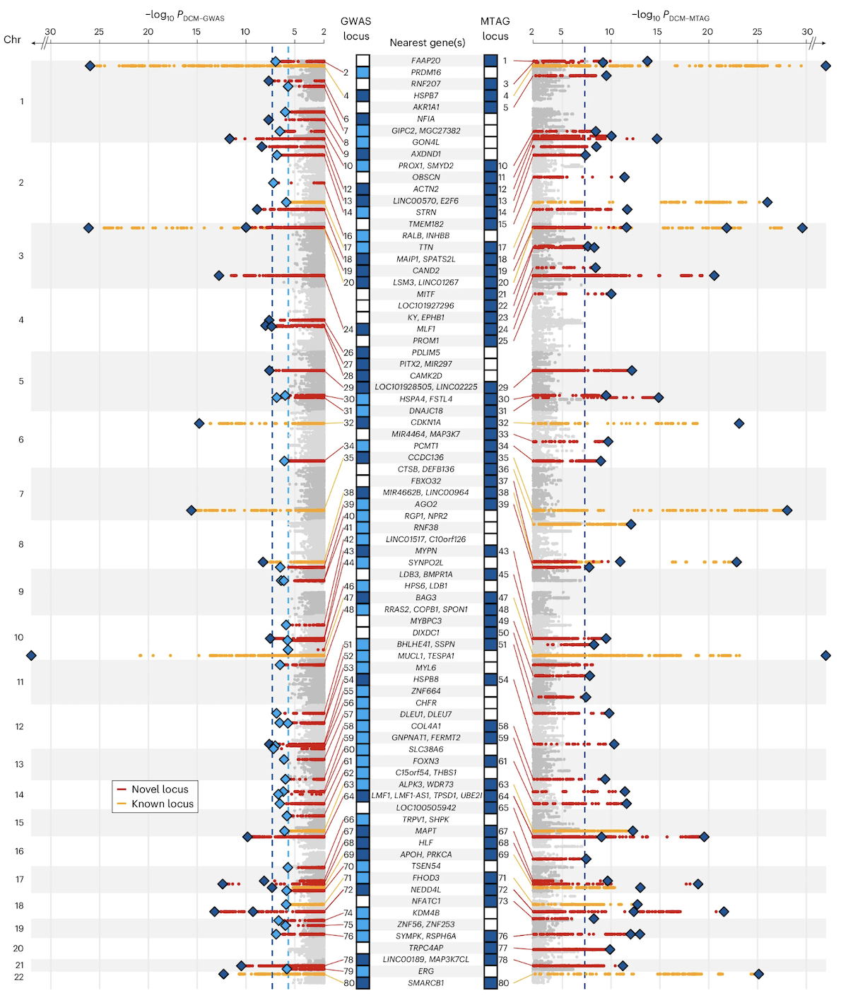
Figure: Manhattan plot of DCM GWAS identifying novel and previously reported genomic loci. Each dot represents a SNP. The y-axis shows −log₁₀(p-value)—higher dots indicate stronger associations. Red peaks mark newly discovered loci, while orange peaks show previously known loci. The significant signals cluster at specific chromosomal regions. These clusters often contain genes involved in the same biological pathways, like muscle structure or cell adhesion. This visualization immediately shows where in the genome the strongest disease associations are located. Source: Zheng, S.L. et al. (2024). Multi-ancestry genome-wide association study of dilated cardiomyopathy. Nature Genetics. https://www.nature.com/articles/s41588-024-01952-y. License: Creative Commons.
Quantile-Quantile (QQ) Plot
The QQ plot is a quality-control tool. It checks whether the distribution of observed p-values matches what you’d expect under the null hypothesis.
Here’s how it works. If none of the SNPs had real effects, all the p-values would follow a uniform distribution—equal numbers of p-values at every level from 0 to 1. On a QQ plot, you plot the expected −log₁₀(p) (what you’d see if all SNPs were null) on the x-axis and the observed −log₁₀(p) (what you actually see) on the y-axis.
If everything is null, the points fall on a diagonal line (y = x). If there are true associations, you’ll see upward deviation at the right tail—the most significant SNPs are more significant than you’d expect by chance. That’s good. It means you found real signals.
But if the entire distribution is shifted upward—not just the tail—that’s a problem. It suggests confounding, often from something called population stratification. This happens when your cases and controls come from different ancestral backgrounds, and the genetic differences between populations create false associations. Modern GWAS methods correct for this using principal components or linear mixed models.
In the DCM study, the QQ plot looked good. Most points fell on the diagonal, with upward deviation only at the tail where the 80 significant loci lived. This confirms the associations are real, not artifacts of confounding.
Together, the Manhattan plot tells you where the associations are, and the QQ plot tells you whether they’re trustworthy.
Biological Interpretation: Pathways, Cell Types, and Functional Convergence
Finding 80 associated loci is exciting, but what does it mean biologically? How do all these scattered SNPs across the genome contribute to heart disease?
This is where pathway enrichment analysis and cell-type analysis come in. The DCM study prioritized 62 candidate genes near the 80 DCM-associated loci and asked: Do these genes share common functions?
The answer was yes. The 62 genes were enriched in pathways related to:
- Muscle structure (sarcomeres, the contractile units of muscle cells)
- Cell adhesion (how heart muscle cells stick together)
- Extracellular matrix (ECM) organization (the scaffolding that holds heart tissue together)
All of these are core components of heart muscle integrity. If the ECM is weak, or if cells can’t adhere properly, the heart can’t contract efficiently—leading to DCM.
Single-nucleus RNA sequencing was also used to see which cell types express these genes. The analysis found that several risk genes are highly expressed in specific cardiomyocyte states (the muscle cells of the heart) and fibroblasts (cells that produce ECM). This cell-type specificity tells you where in the heart the genetic risk plays out.
This is an example of functional convergence. Even though the 80 loci are scattered across the genome, they participate in shared biological pathways. It’s like having 80 different entry points into the same building—they all lead to the same place.
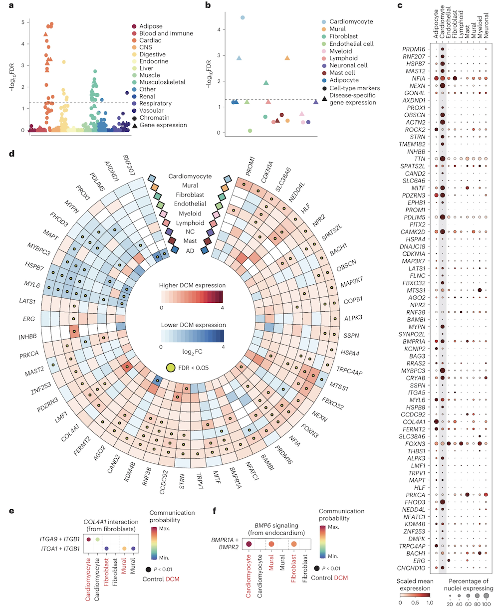
Figure: Enrichment of prioritized DCM genes across pathways and cell types. This figure shows which biological pathways and cell types are enriched for DCM candidate genes. Pathways related to cardiac structure and ECM dominate, and specific cardiomyocyte and fibroblast states light up. Despite the complexity—many loci, many genes—the biological story is coherent: these genes converge on mechanisms that maintain heart muscle structure. That’s how a polygenic trait produces a unified disease phenotype. Source: Zheng, S.L. et al. (2024). Multi-ancestry genome-wide association study of dilated cardiomyopathy. Nature Genetics. https://www.nature.com/articles/s41588-024-01952-y. License: Creative Commons.
Polygenic Scores (PGS)
We’ve found 80 loci associated with DCM. Each locus contributes a tiny bit to disease risk. How do we combine all that information into something useful for an individual person?
That’s where polygenic scores (PGS) come in. A polygenic score—also called a polygenic risk score or genomic score—quantifies your cumulative genetic risk by summing up the effects of all your risk alleles.
Here’s how it works. For each of the 80 DCM-associated SNPs, the GWAS tells you the effect size—how much that SNP increases risk. You check which alleles the person carries at those SNPs, multiply by the effect sizes, and add them all up. The result is a single number representing that person’s genetic liability for DCM.
Polygenic scores are especially valuable for complex traits, where no single mutation determines the outcome. Instead of looking at one gene, you’re integrating information from thousands of variants across the genome.
Example: Dilated Cardiomyopathy (DCM)
In the DCM study, a PGS for DCM was calculated using the 80 significant loci. Then the score was tested in the UK Biobank—a huge dataset of about 500,000 people with genetic and health records.
Here’s what was found:
Individuals in the top 10% of PGS had a 2.8-fold higher risk of developing DCM compared to those in the lowest 10%. That’s nearly three times the risk, just from common genetic variants.
This elevated risk held even in people without rare pathogenic mutations. In other words, your polygenic background matters even if you don’t carry a known disease-causing mutation.
But here’s the really interesting part: among people who do carry pathogenic variants—like mutations in TTN or LMNA, which are known causes of cardiomyopathy—those with high PGS were significantly more likely to develop DCM than carriers with low PGS.
This shows that polygenic background modifies penetrance. Having a rare mutation doesn’t guarantee you’ll get the disease. Your polygenic score acts as a modifier, tipping you toward or away from clinical disease.
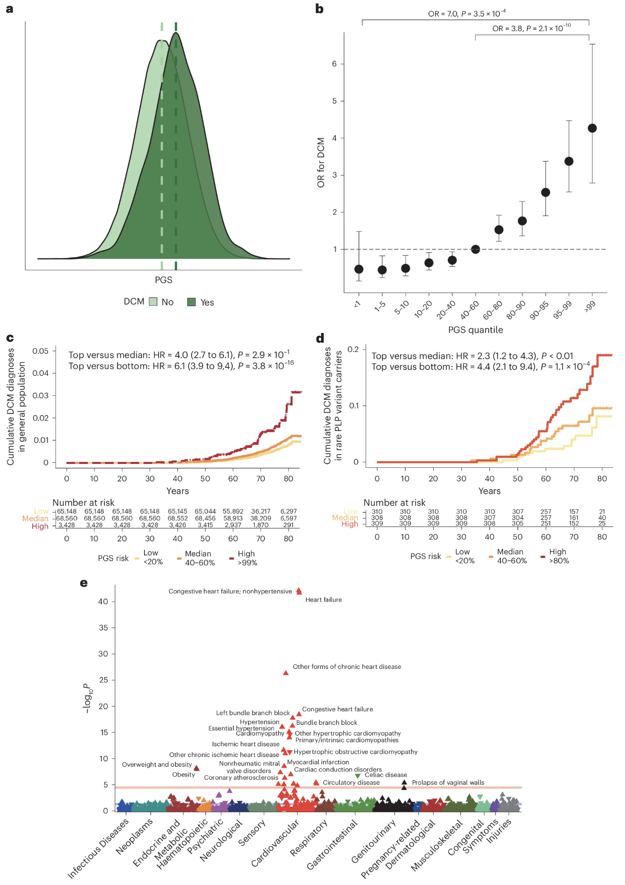
Figure: DCM PGS is associated with DCM disease status in the UK Biobank. The prevalence of DCM increases steadily as you move from the lowest PGS decile (left) to the highest (right). People in the top 10% have about 2.8 times the risk of those in the bottom 10%. The dark bars represent carriers of rare pathogenic variants, while lighter bars represent non-carriers. Notice that even among pathogenic variant carriers, higher PGS predicts higher disease prevalence. This demonstrates that polygenic background affects penetrance—even in what we used to think of as “monogenic” diseases. Source: Zheng, S.L. et al. (2024). Multi-ancestry genome-wide association study of dilated cardiomyopathy. Nature Genetics. https://www.nature.com/articles/s41588-024-01952-y. License: Creative Commons.
Application of Polygenic Scores
Polygenic scores are moving from research tools to clinical applications. Here are some of the ways they’re being used:
Risk prediction and early detection. If you have a high PGS for heart disease, you might benefit from earlier cardiac screening—echocardiograms, stress tests, and so on. You can also take preventive measures like improving diet, exercising more, or monitoring blood pressure closely. The goal is to catch problems before they become serious.
Precision medicine. Combining PGS with rare variant data gives a more complete picture of genetic risk. If you carry a pathogenic mutation and have a high PGS, your doctor knows you’re at especially high risk and can adjust treatment accordingly. Genetic counselors can use this information to give more accurate risk estimates.
Population research. PGS lets studies investigate how genetic architecture varies across populations. For example, does the genetic basis of height differ between Europeans and East Asians? How do genetic risk factors interact with environmental exposures like diet or pollution? PGS provides a quantitative measure of genetic liability that can be compared across groups.
Drug discovery. Genes contributing to polygenic risk often point to biological pathways that could be targeted with drugs. If many DCM risk genes are involved in ECM organization, maybe drugs that strengthen the ECM could help. GWAS and PGS can guide where to look for new therapies.
These applications show how GWAS findings extend beyond discovery. They’re becoming tools for actionable insights in clinical and translational genomics.
Ethical Considerations in the Use of Polygenic Scores
Polygenic scores hold great promise, but they also raise serious ethical questions. We need to think carefully about how we use this technology.
Equity and ancestry bias. Most GWAS datasets are heavily European. As of 2024, more than 80% of GWAS participants have European ancestry. This means polygenic scores trained on European data often don’t work well in other populations. If you apply a European-derived PGS to someone of African or East Asian ancestry, the predictions can be wildly inaccurate. This creates health disparities—people from underrepresented populations don’t benefit equally from genomic medicine. The solution is to include more diverse participants in GWAS, but that’s still a work in progress.
Privacy and data protection. Genetic data are uniquely identifying. Your genome is like a fingerprint, but even more personal—it reveals information about your relatives too. If genetic data leak or are misused, the consequences can be severe. Strict safeguards are needed to protect against breaches, especially as genomic databases grow.
Interpretation and communication. A high polygenic score means increased probability of disease, not certainty. If your PGS puts you in the top 10% for heart disease risk, that doesn’t mean you’ll definitely get heart disease. It means your baseline risk is higher than average. Clinicians need to communicate this distinction clearly. Patients need to understand that genetics is one factor among many—lifestyle, environment, and luck all matter too.
Psychological and social impacts. Learning you have high genetic risk can be distressing. It might affect your mental health, self-perception, or life decisions. Would you want to know if you’re at high risk for Alzheimer’s disease, knowing there’s currently no cure? Different people answer that question differently. There’s also a risk of genetic stigma—being treated differently because of your genes, whether by insurers, employers, or even family members.
Regulatory oversight. As polygenic scores move into clinical use, we need clear policies governing how they’re used. Should insurance companies be allowed to use PGS in risk assessment? Should employers have access to genetic data? Most countries have laws against genetic discrimination, but enforcement and scope vary. We need transparent, fair policies that balance the benefits of genomic medicine with protection of individual rights.
These considerations remind us that science doesn’t exist in a vacuum. Polygenic scores are powerful tools, but they must be applied responsibly. The technology is advancing faster than our ability to handle its ethical implications, so ongoing dialogue between scientists, clinicians, policymakers, and the public is essential.
Putting It All Together
Let’s recap what we’ve learned about GWAS and polygenic scores.
GWAS identifies common genetic variants associated with traits by testing millions of SNPs across the genome. It compares allele frequencies between cases and controls and uses stringent statistical thresholds to avoid false positives. The result is a list of genomic loci that contribute to the trait.
We visualize GWAS results using Manhattan plots (showing where the associations are) and QQ plots (validating that they’re real). These plots help us make sense of millions of data points and catch potential confounding.
Pathway and cell-type analyses reveal functional convergence—showing that dispersed loci often act through shared biological mechanisms. For DCM, 80 scattered loci converged on pathways related to muscle structure, cell adhesion, and ECM. This tells us how genetic variation leads to disease.
Polygenic scores quantify additive genetic risk by combining the effects of many variants into a single number. They enable practical applications in risk prediction, precision medicine, and drug discovery. The DCM example showed that PGS can identify high-risk individuals and modify penetrance even in carriers of rare pathogenic mutations.
But with great power comes great responsibility. Ethical challenges—ancestry bias, privacy, interpretation, psychological impacts, and regulatory oversight—must be addressed as genomics moves from research to real-world implementation. We need to ensure that genomic medicine is not only scientifically valid but also socially fair.
GWAS has transformed our understanding of complex traits. It confirmed Fisher’s century-old polygenic model and revealed the genetic architecture of thousands of traits and diseases. As datasets grow and methods improve, GWAS will continue to drive discoveries—but we must remain vigilant about how we apply those discoveries in society.