human genetics
Part 3. Polygenic Genetics and Complex Traits: From Single Genes to Genomic Landscapes
Introduction: When Mendel’s Laws Meet Thousands of Genes
In Part 2, you learned how Mendel’s laws apply to single genes—how one mutation in CFTR causes cystic fibrosis, how KMT2D haploinsufficiency causes Kabuki syndrome, how recessive inheritance requires two mutant alleles. These are clean stories: one gene, clear mechanism, predictable inheritance.
But most traits don’t work this way. Height isn’t controlled by one gene. Neither is heart disease, diabetes, or intelligence. These traits show continuous variation—smooth bell curves, not discrete categories. They run in families, suggesting genetic influence, yet don’t follow Mendel’s 3:1 ratios.
This paradox puzzled early geneticists. On one side were the Mendelians, who studied discrete traits like pea color that came in clear categories and followed simple ratios. On the other side were the biometricians, who measured continuous traits like height that showed smooth variation and no obvious Mendelian patterns. The two groups thought they were studying fundamentally different phenomena.
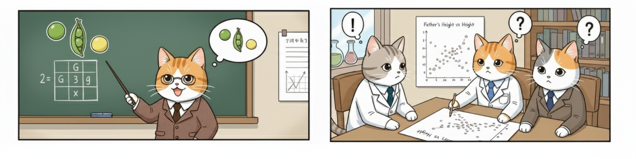
Left: Mendelian genetics explains discrete traits (green vs yellow peas) with clear ratios. Right: Continuous traits like height show smooth parent-offspring correlations without obvious categories—leaving early geneticists puzzled.
In 1918, statistician R.A. Fisher resolved this paradox with a simple insight: continuous variation can arise from many genes, each following Mendel’s laws, each contributing a small additive effect. If hundreds of loci affect height, and you inherit random combinations from your parents, the result is a bell curve—not because inheritance has changed, but because you’re summing many independent Mendelian factors.
Fisher couldn’t prove this directly. He worked with mathematics and trait correlations between relatives, deducing that many genes must exist because that’s what the data required. For 80 years, his model remained elegant theory.
Then came genome-wide association studies (GWAS). We scanned millions of variants across hundreds of thousands of people and found Fisher was right: height is influenced by over 12,000 genetic variants across the genome. Type 2 diabetes involves hundreds of loci. Schizophrenia has 287 associated regions. Each variant has a tiny effect—shifting phenotype by milligrams or millimeters—but together they explain substantial heritability.
This chapter shows how Mendel’s laws scale from single genes to genomic complexity, how we find and interpret thousands of small-effect variants, and why the same disease can arise through completely different genetic routes that converge on shared biology.
What This Chapter Is About
This chapter has six interconnected sections explaining how we interpret complex genetic architecture:
1. Additive vs. Dominant Alleles
How do alleles combine their effects? Using height as our model, we’ll contrast dominant disorders (achondroplasia, Marfan syndrome) where one mutation has a large effect, with normal variation where thousands of additive variants each contribute tiny amounts. You’ll understand why most traits show predominantly additive effects—and what “orthogonalized dominance” means when testing this.
2. Heritability: What It Means and What It Doesn’t
What does “height is 68% heritable” actually mean? This section tackles genetics’ most misunderstood concept. Using Fisher’s framework and modern twin/SNP studies, you’ll learn why heritability measures population variance (not individual determination), why it changes across environments, and why high heritability doesn’t mean traits are fixed or that environment doesn’t matter.
3. Variance Partitioning in Practice
How does partitioning genetic and environmental variance answer biomedical questions? We’ll examine two recent studies: one showing the gut microbiome doesn’t cause autism (it reflects dietary preferences), another showing prenatal acetaminophen doesn’t cause autism (the association was due to familial confounding). Both demonstrate why properly accounting for shared genetic and environmental factors is essential for causal inference.
4. Genome-Wide Association Studies (GWAS)
How do we actually find the thousands of variants influencing complex traits? You’ll learn how GWAS works, how to read Manhattan and QQ plots, what genome-wide significance (p < 5×10⁻⁸) means and why it’s necessary, and how researchers translate statistical associations into biological understanding through pathway and cell-type analyses. We’ll also cover polygenic scores—combining thousands of tiny effects into risk predictions.
5. Genetic Architecture of Complex Diseases
Why do different people develop the same disease through different genetic routes? Using dilated cardiomyopathy, Alzheimer’s disease, and autism as examples, you’ll see how diseases have composite genetic architecture—rare high-impact mutations in some patients, polygenic risk in others, or combinations of both. Despite genetic heterogeneity, variants often converge on shared biological pathways.
6. From Statistics to Mechanism
How do we connect GWAS loci to causal biology? This section shows how statistical associations point to specific genes, pathways, and cell types. You’ll understand the difference between a GWAS locus (a chromosomal region) and the actual causal variant, why most associations are in non-coding regions, and how functional studies validate predicted mechanisms.
From Pea Ratios to Polygenic Scores
Consider type 2 diabetes—a complex metabolic disease. The traditional view:
- Runs in families (genetic component)
- Influenced by diet and exercise (environmental component)
- No clear Mendelian pattern (not a single-gene disorder)
- Mechanism unclear (polygenic? environmental? both?)
The modern genomic view:
- GWAS identifies ~400 associated loci across the genome
- Each variant increases risk by 1-10% (tiny individual effects)
- Polygenic score combining all loci predicts ~5-fold risk difference between top and bottom deciles
- Rare monogenic forms exist (MODY, neonatal diabetes) but represent <5% of cases
- Common and rare variants affect same pathways: insulin secretion, glucose metabolism, beta-cell function
- Confirmation: most diabetes is polygenic, but specific genes/pathways are identifiable
This is still Mendelian inheritance at each locus—alleles segregate according to Mendel’s laws. But now we observe:
- Thousands of loci simultaneously
- How tiny effects combine into substantial risk
- Why family history predicts risk (shared polygenic background)
- How rare and common variants interact
- Which biological pathways matter
This chapter focuses on complexity: moving from single-gene thinking to genomic-scale interpretation.
How to Approach This Chapter
Think Additively, Not Categorically
Most genetic effects are additive. Two copies of a risk allele ≈ twice the effect of one copy. This seems simple, but it has profound implications:
- Traits show continuous variation (bell curves)
- Many genes of small effect can produce large phenotypic differences
- Family resemblance reflects shared polygenic background
- Dominance effects are rare and weak for most traits
Understand What Heritability Does and Doesn’t Tell You
“Height is 68% heritable” means:
- 68% of height variation in this population is due to genetic variation
- NOT: 68% of your height is genetic (that’s meaningless)
- NOT: height is 68% determined by genes (ignores gene-environment interplay)
- NOT: environment only matters 32% (heritability changes with environment)
Heritability is a population statistic, not an individual property.
Connect Multiple Evidence Streams
Interpreting complex traits requires integrating:
- GWAS: Which loci are associated? (statistical evidence)
- Functional studies: What do these genes do? (biological mechanism)
- Pathway analysis: Do variants converge on shared biology? (functional coherence)
- Cell-type enrichment: Where do these genes act? (tissue specificity)
- Polygenic scores: What’s the cumulative effect? (predictive power)
- Rare variants: Are there high-impact mutations too? (genetic architecture)
No single analysis suffices. Complex traits require comprehensive approaches.
Recognize the Spectrum
Traits aren’t purely Mendelian or purely polygenic—they exist on a continuum:
- Height: mostly polygenic, some monogenic cases (achondroplasia, Marfan)
- Autism: mostly polygenic, ~10-20% monogenic (CHD8, SCN2A, fragile X)
- Alzheimer’s: mostly polygenic, rare early-onset forms (APP, PSEN1/2)
- Coronary artery disease: mostly polygenic, rare monogenic (familial hypercholesterolemia)
The same trait can follow different genetic rules in different individuals.
What Makes This Different From Mendelian Genetics
| Mendelian Approach | Polygenic Approach |
|---|---|
| Single gene, large effect | Thousands of genes, tiny effects |
| Discrete categories (affected/unaffected) | Continuous variation (bell curves) |
| Clear inheritance patterns (3:1 ratios) | Familial clustering without simple ratios |
| High penetrance (mutation → disease) | Low penetrance (risk alleles increase probability) |
| Study rare families with clear segregation | Study large populations with subtle associations |
| One mutation explains phenotype | Thousands of variants contribute to phenotype |
| Predict from single genotype | Predict from polygenic score |
Both frameworks are valid—they describe different ends of the genetic architecture spectrum.
Learning Objectives
By the end of this chapter, you should be able to:
-
Explain Fisher’s insight that continuous traits arise from many genes with small additive effects, and understand how this unified Mendelian and biometric perspectives
-
Distinguish additive from dominant alleles using molecular mechanisms and population data, and understand why most effects are additive
-
Interpret heritability correctly as a population statistic measuring variance components, not as individual genetic determination
-
Apply variance partitioning to distinguish correlation from causation in observational studies, recognizing how shared genetic and environmental factors create confounding
-
Read and interpret GWAS results including Manhattan plots, QQ plots, pathway enrichment, and cell-type analyses
-
Calculate and understand polygenic scores, including their construction, interpretation, limitations, and ethical implications
-
Describe genetic architecture of complex diseases, recognizing that rare and common variants can contribute to the same phenotype through convergent pathways
-
Connect GWAS associations to biological mechanisms by integrating statistical evidence with functional studies, pathway analyses, and cell-type data
Let’s Begin
Part 2 showed you how to interpret single variants—determining whether a mutation causes disease, understanding dominance mechanisms, applying Mendel’s laws to sequence data.
Part 3 shows you how to interpret thousands of variants simultaneously—understanding how tiny effects combine, why traits show continuous variation, and how different genetic routes can produce the same disease.
Fisher predicted in 1918 that many genes of small effect must exist. GWAS proved him right a century later. Now you’ll learn how to find those genes, interpret their effects, and understand the complex genetic architecture underlying most human traits and diseases.
Mendel gave us the rules for single genes. Fisher showed how those rules scale to thousands of genes. Modern genomics makes both frameworks visible in sequence data.
Let’s see how genetic complexity emerges from simple principles.