Chapter 60. Thermodynamic RNA Secondary-Structure Prediction and Zuker-Style Algorithms
Scope Note
Thermodynamic RNA secondary-structure prediction asks a narrowly defined but biologically influential question: given an RNA sequence and an energy model, which base-pairing pattern is expected to have the lowest free energy under the model’s assumptions? This chapter focuses on minimum-free-energy prediction, Zuker-style dynamic programming, nearest-neighbor parameters, practical constraints, loop energetics, benchmarking, and reproducible software use. Probabilistic partition functions, base-pair probabilities, pseudoknot-specialized algorithms, comparative covariation, probing-constrained integrative modeling, tertiary modeling, and inverse design are introduced only where needed and are treated more fully in Chapters 61 to 65.
Executive Summary
RNA secondary-structure prediction is usually a prediction of canonical and wobble base pairs arranged into stems, loops, bulges, internal loops, and multibranch loops. The common thermodynamic version of the problem assigns free-energy contributions to local motifs, then searches for the non-pseudoknotted structure with the minimum total free energy. Dynamic programming makes that search tractable by decomposing a long sequence into overlapping intervals, calculating optimal solutions for smaller intervals, and reusing those solutions when evaluating larger intervals. This decomposition is the computational reason that a sequence with astronomically many possible foldings can be analyzed in seconds or minutes, provided the algorithm restricts the structure class and uses an energy model that can be evaluated recursively.
The Zuker-style algorithmic tradition is more specific than “predict the best RNA fold.” It combines dynamic programming recursions with a nearest-neighbor thermodynamic model and a formal trace-back procedure that returns one or more low-energy secondary structures. The nearest-neighbor model treats the stability of a helix as depending on adjacent base pairs, loop type, loop size, terminal mismatches, dangling bases, and selected special motifs. This model is empirical. Its parameters come from optical melting and related thermodynamic measurements on defined RNA oligonucleotides, then are generalized to longer RNAs. The result is useful, but it is not a complete physical theory of RNA folding in cells.
The minimum-free-energy structure is best understood as a model-dependent hypothesis, not as the observed biological structure. A single RNA sequence can have many structures close in free energy. Cellular folding can be co-transcriptional and kinetic rather than fully equilibrated. Proteins, ions, ligands, modifications, ribosomes, helicases, and degradation pathways can select structures that differ from the in vitro equilibrium prediction. Even within the thermodynamic model, multibranch loops, dangling ends, coaxial stacking, noncanonical contacts, modified nucleotides, and pseudoknots are only partly represented. Prediction is therefore strongest for compact RNAs with well-parameterized local motifs and weakest for long, dynamic, protein-bound, pseudoknotted, heavily modified, or context-dependent RNAs.
Benchmarking should compare a predicted base-pair set with an experimentally supported reference structure, but the reference itself is often uncertain. Crystal, cryo-EM, NMR, chemical probing, comparative covariation, and mutational evidence measure different aspects of RNA structure. A benchmark can reward a model for matching a deposited secondary structure while missing alternative conformations or condition-dependent states. Conversely, a prediction can be biologically useful even when it is not the single annotated native structure, especially if it identifies stable local elements, competing folds, or regions where the energy model is indecisive. Recent reviews and comparative analyses treat thermodynamic folding as one important member of a broader software ecosystem that now includes machine-learning, hybrid, comparative, and experimentally constrained methods.
Concept Inventory
- Secondary structure: the set of intramolecular base pairs usually represented without full three-dimensional coordinates. In thermodynamic prediction, secondary structure most often includes Watson-Crick G-C and A-U pairs plus G-U wobble pairs, arranged without pseudoknots unless a specialized algorithm says otherwise. Noncanonical pairs, base triples, metal-mediated contacts, and tertiary docking can be biologically important but are usually outside the basic Zuker-style model.
- Minimum free energy: the lowest Gibbs free energy structure found under a chosen energy model and allowed structure class. MFE is not synonymous with “native structure.” It is the optimum of a model. If the model omits a ligand, protein, modification, pseudoknot, salt condition, or kinetic pathway, the MFE structure can be a correct mathematical answer to an incomplete biological question.
- Dynamic programming: an algorithmic strategy that breaks a problem into smaller overlapping subproblems and stores their solutions. In RNA folding, the subproblem is often “what is the best structure for the interval from nucleotide i to nucleotide j under a specified boundary condition?” The boundary condition matters because an interval can be unpaired, closed by a base pair, part of a multibranch loop, or constrained by neighboring choices.
- Nearest-neighbor thermodynamics: the empirical assumption that local RNA stability can be approximated by adding parameters for neighboring base-pair stacks and loop motifs. The phrase “nearest neighbor” is clearest for helices, where the free energy of a stacked pair depends on the identities of two adjacent base pairs. The full folding model also includes loop initiation penalties, mismatch terms, dangling ends, special hairpin motifs, multiloop penalties, and sometimes coaxial stacking.
- Zuker-style algorithms: dynamic-programming algorithms that compute optimal or near-optimal RNA secondary structures using a thermodynamic energy model. The term refers to a family of recursions and software lineages rather than one frozen implementation. Different packages vary in parameter sets, treatment of dangling ends, suboptimal enumeration, constraints, multiloop models, and output conventions.
- Hard constraints: forbid or require structural features. A hard constraint might require nucleotide 20 to pair with nucleotide 85, prohibit nucleotide 42 from pairing, or force a region to remain single stranded. Soft constraints change energies without absolutely forbidding alternatives. Chemical-probing pseudoenergies are common soft constraints: reactive nucleotides can be penalized if predicted paired, while less reactive positions are treated more cautiously.
- Suboptimal structures: structures whose computed energies are close to, but not necessarily equal to, the MFE structure. They matter because a small free-energy difference may be smaller than parameter uncertainty, biological fluctuations, or omitted environmental effects. A low-energy ensemble of alternatives can be more informative than a single optimum when an RNA has competing regulatory folds.
What to Know Before Reading This Chapter
Readers should be comfortable with three background ideas. First, RNA is a single-stranded polymer with directional polarity, commonly written from 5′ to 3′. The bases A, C, G, and U can pair intramolecularly, and contiguous base pairs form helices. Second, Gibbs free energy describes the thermodynamic favorability of a state; lower free energy is more stable at equilibrium under specified conditions. Third, a computer algorithm can be scientifically useful without being biologically complete. A folding program solves a formal problem defined by inputs, allowed structures, parameter values, and output rules.
The running examples in this chapter are a bacterial riboswitch aptamer, a messenger RNA 5′ untranslated region, a viral RNA regulatory element, and an engineered small RNA. A riboswitch aptamer shows why ligand binding and alternative folds complicate pure sequence-to-MFE prediction. A 5′ untranslated region shows why local structure can affect translation but also why ribosomes and RNA-binding proteins change the relevant question. A viral RNA element shows why long-range pairings and pseudoknots can exceed the basic model. An engineered small RNA shows how thermodynamic folding supports design but requires reproducible software, parameter, and constraint reporting.
This chapter uses “prediction” in a restrained sense. A predicted structure is a proposed base-pairing model. It becomes evidence for biology only after comparison with experimental data, conservation, perturbation, or functional readouts. Chapter 59 explains structural and biophysical evidence; Chapter 63 explains probing constraints; Chapter 61 explains ensembles and base-pair probabilities; Chapter 62 explains comparative evidence.
60.1. Dynamic programming and MFE recursion
The central challenge in RNA secondary-structure prediction is combinatorial. Even a modest RNA sequence can fold into an enormous number of possible base-pairing patterns. Exhaustively drawing every possible structure and scoring each one is impossible for ordinary biological sequences. Dynamic programming solves this by exploiting a property of many secondary-structure energy models: the energy of a larger structure can be computed from energies of smaller pieces plus a local term for the loop or pair that connects them.
Consider a sequence interval from nucleotide i to nucleotide j. A simple algorithm asks whether nucleotide i is unpaired or paired with some nucleotide k between i plus a minimum loop distance and j. If i is unpaired, the best structure on i through j depends on the best structure on i+1 through j. If i pairs with k, the algorithm adds the score for the pair or the loop closed by that pair, then combines it with the best structures on the remaining intervals. More realistic algorithms use several matrices because the energy contribution depends on context: a base pair closing a hairpin loop is different from a pair closing an internal loop, and both are different from a pair inside a multibranch loop.
The term recursion means a rule that defines the value of a larger interval in terms of values already calculated for smaller intervals. For RNA folding, the values are free energies. The recursions are evaluated in an order that ensures smaller intervals are known before larger intervals need them. Once the dynamic-programming tables are filled, a trace-back step reconstructs the choices that produced the lowest energy. The output can be a set of base pairs, a dot-bracket string, and a computed free energy.
Table 60.1. Thermodynamic Terms and Their Caveats. Major energy terms in nearest-neighbor RNA folding. The model is strongest for experimentally parameterized local motifs and weaker for modified bases, protein-bound states, tertiary coupling, and poorly sampled junction geometries.
| Term | Structural Feature | Evidence Basis | Where Reliable | Common Caveat |
|---|---|---|---|---|
| Base-pair stack | Adjacent paired bases in a helix | Optical melting of RNA duplexes | Short canonical helices | Less accurate near helix termini or with modified bases |
| Hairpin-loop initiation | Single-stranded loop closing a stem | Melting of hairpin oligomers | Loops of 4–8 nt with canonical closing pairs | Special stable tetraloops require separate parameters |
| Terminal mismatch | Unpaired bases at a helix end inside a loop | Measured on short duplexes | Well-sampled mismatch identities | Less reliable for rare or modified terminal identities |
| Internal loop | Unpaired nucleotides on both strands of a helix | Melting of loop-containing duplexes | Symmetric loops of moderate size | Large or asymmetric loops poorly parameterized |
| Bulge | Unpaired nucleotides on one strand of a helix | Melting of bulge-containing constructs | Single-nucleotide bulges | Multi-nucleotide bulges are approximated |
| Multibranch loop | Junction of three or more helices | Inferred indirectly; few direct measurements | Simple linear approximation used broadly | Poorly parameterized; simpler models can outperform complex ones |
| Dangling end | Unpaired base stacking on a helix terminus | Melting of duplexes with single-stranded overhangs | Single dangling nucleotides | Program-dependent treatment can change predicted energies |
| Special stable loop motif | Specific tetraloop or hexaloop sequences | Direct thermodynamic measurement | GNRA and UNCG tetraloops | Scope limited to characterized sequences |
| Coaxial stacking | End-to-end helix alignment across a junction | Inferred from structural and melting data | Favorable junction geometries | Difficult to predict from sequence alone |
| Constraint pseudoenergy | Soft penalty from chemical probing reactivity | Empirical calibration from probing experiments | Well-probed single-conformation RNAs | Reactivity can reflect protein binding or poor reagent access |
Table 60.2. Reproducibility Checklist for RNA Folding Predictions. A folding prediction is reproducible only when the formal problem is fully documented. Sequence boundaries, software version, parameter set, temperature, constraints, dangle model, and suboptimal settings can all change the predicted structure or its interpretation.
| Item | Example | Why It Matters |
|---|---|---|
| Sequence and coordinates | NCBI accession NM_001234, positions 1–250 | Ambiguous boundaries change the predicted structure |
| Molecule state | Mature spliced mRNA; 5′ UTR only | Folding context differs for precursor versus processed RNA |
| Software and version | RNAfold 2.6.4; RNAstructure 6.4 | Defaults and algorithms differ across versions |
| Parameter set | Turner 2004; NNDB 2022 | Different parameter sets can reorder competing folds |
| Temperature | 37 °C (default); 25 °C for in vitro assay | Enthalpy-entropy balance shifts with temperature |
| Constraints | SHAPE pseudoenergies; required base pair | Constraints change the formal problem being solved |
| Dangle settings | —dangles 2 (RNAfold default) | Dangle treatment alters energies, especially for short RNAs |
| Suboptimal method | Energy window 5 kcal/mol; stochastic sampling | Different methods return different alternative sets |
| Selected output | First returned structure; structure closest to probing data | Selection criteria affect biological interpretation |
| Command or workflow file | Shell script archived in project repository | Enables exact replication by other laboratories |
A minimal pedagogical recursion is not the same as a production RNA folding algorithm. Real implementations must handle hairpin-loop initiation, interior loops with two unpaired sides, bulges with one unpaired side, stacked pairs, terminal mismatches, dangling bases, multibranch loops, coaxial stacking options, constraints, and tie-breaking rules. The mathematical structure remains the same: local choices are scored, compatible substructures are combined, and the program avoids recomputing the same interval repeatedly. Reviews of RNA secondary-structure prediction describe this dynamic-programming foundation as the historical backbone on which later thermodynamic, comparative, and hybrid methods were built.
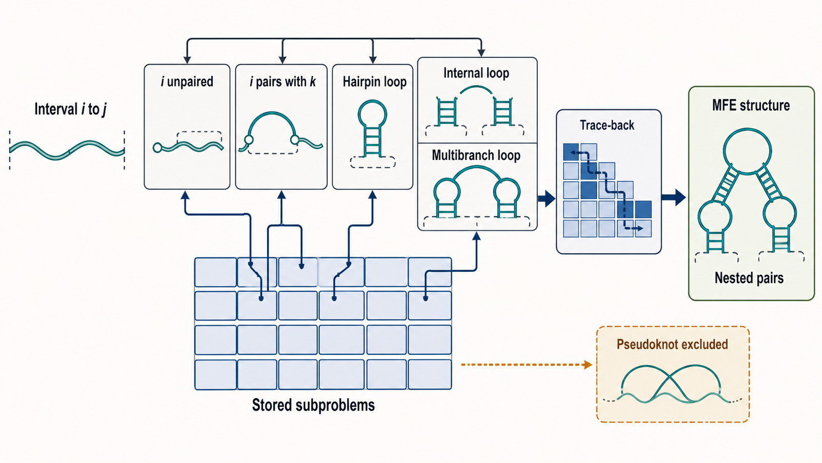
Figure 60.1. Dynamic-Programming Recursion for MFE Folding. Dynamic programming turns RNA MFE folding from an impossible exhaustive search into a recursion over sequence intervals. For an interval i through j, the algorithm evaluates cases such as nucleotide i being unpaired, nucleotide i pairing with k, or a closing pair defining a hairpin, internal loop, bulge, or multibranch loop. Previously calculated smaller intervals are reused, and a trace-back step reconstructs the lowest-energy base-pairing pattern. Ordinary nested recursion excludes crossing pseudoknot pairs, which require specialized algorithms.
The simplest important restriction is that standard Zuker-style folding excludes pseudoknots. A pseudoknot occurs when base pairs cross in sequence order, such as i pairing with k and j pairing with l where i < j < k < l. Noncrossing base pairs can be represented as nested intervals, which dynamic programming handles efficiently. Crossing base pairs break that interval decomposition. Some algorithms predict restricted pseudoknot classes, but the general problem is harder and belongs primarily to Chapter 61 and specialized pseudoknot treatments.
MFE recursion also assumes that the RNA has equilibrated under the parameterized conditions. This is not always true. Co-transcriptional folding can trap a structure before the full sequence is available. A riboswitch expression platform may choose between mutually exclusive terminator and antiterminator helices while RNA polymerase is still transcribing. A viral RNA genome may be packaged with proteins that stabilize a non-MFE conformation. A therapeutic small RNA may be designed so the intended duplex or hairpin is stable under formulation conditions, but cellular proteins and modifications still change its folding landscape. MFE prediction is therefore a disciplined baseline, not a complete model of intracellular RNA folding.
The most useful way to read an MFE result is to ask what formal question was answered. Was the sequence folded as one long molecule or in sliding windows? Were temperature and salt assumptions defaults? Were modified nucleotides ignored? Were base pairs constrained by probing data? Were alternative low-energy structures requested? Were pseudoknots prohibited? A predicted free energy without those details is not reproducible and should not be compared quantitatively with another prediction.
Box 60.1. Common Overinterpretations of MFE Predictions
- The MFE structure is the lowest-energy solution under the model, not necessarily the cellular native structure.
- A low computed free energy is not evidence of biological function or cellular occupancy.
- A missing pseudoknot in a standard fold is not evidence that the pseudoknot is absent; ordinary dynamic programming cannot represent crossing pairs.
- A probing-constrained prediction is a model informed by reactivity data, not a direct structure determination.
- Deep-learning predictions still require experimental validation outside their training distribution.
- Software package defaults vary; the same sequence can yield different structures in different programs or versions.
60.2. Zuker-style algorithms and suboptimal structures
Zuker-style algorithms are the canonical thermodynamic approach to single-sequence RNA secondary-structure prediction. The core aim is to find the lowest-energy secondary structure in a defined class, usually non-pseudoknotted structures with allowed canonical and G-U base pairs. The phrase “Zuker-style” also signals a practical software tradition: algorithms that use experimentally derived thermodynamic parameters, loop-specific recursions, trace-back, and optional enumeration of low-energy alternatives. Mathews’s historical review remains a useful guide to why this approach shaped the field and how later improvements emerged.
The causal logic of a Zuker-style fold can be described in five steps. First, the input sequence is parsed and possible base pairs are identified according to allowed pairing rules and minimum loop sizes. Second, dynamic-programming tables are filled with optimal energies for intervals under different structural states. Third, the program evaluates loop types using a thermodynamic parameter set. Fourth, trace-back reconstructs the decisions that produced the MFE structure. Fifth, optional routines generate suboptimal structures, energy dot plots, or constraint-aware alternatives. Each step has biological consequences. For example, changing the allowed pair set can alter predicted helices; changing the parameter set can reorder competing folds; changing the suboptimal-energy window can change which alternatives a user sees.
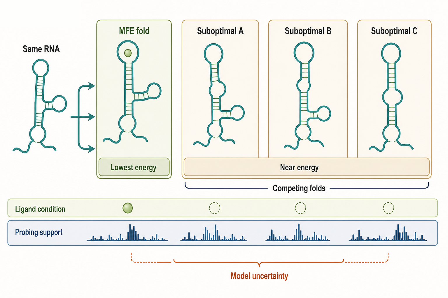
Figure 60.2. MFE and Suboptimal Structures for a Riboswitch-Like RNA. A riboswitch-like leader RNA can have several low-energy folds. The MFE structure is the lowest computed energy state under the model, but near-optimal alternatives can represent regulatory competitors or parameter uncertainty. Experimental evidence such as ligand-dependent probing, transcription readthrough, and compensatory mutations is needed to decide which fold is occupied in a biological condition.
Suboptimal prediction is not an afterthought. Many RNAs have several folds within a few kcal/mol of the MFE structure. That energy spacing can be comparable to uncertainty in thermodynamic parameters or to stabilizing effects from one protein, ligand, or ion. A riboswitch leader RNA can have a ligand-bound aptamer fold and a mutually exclusive expression-platform fold. A viral RNA element can use alternative long-range interactions in different replication or translation states. A messenger RNA region can expose or hide an initiation site depending on translation, RNA-binding proteins, and local unfolding. In each case, a ranked list of near-optimal structures is often more biologically useful than one optimum.
Different programs define “suboptimal” differently. Some enumerate all structures within an energy increment of the MFE subject to limits. Some sample structures from a thermodynamic ensemble, which is more properly a Chapter 61 topic. Some produce local alternatives by forcing different helix choices. Some report a representative set to avoid overwhelming redundancy. Users should therefore specify the software, version, parameter set, temperature, constraint file, and suboptimal-generation mode. Without those details, two laboratories can both say “we predicted suboptimal structures” while performing different computations.
Tie-breaking is another underappreciated issue. Two structures can have identical or nearly identical computed energies. A program may return one because of matrix traversal order, implementation detail, or an arbitrary preference. A user who treats the first returned structure as uniquely meaningful can overinterpret a numerical tie. Dot plots, suboptimal lists, and base-pair probabilities help reveal such ambiguity. Even when this chapter focuses on MFE, the practical lesson is that thermodynamic prediction should report uncertainty whenever the energy landscape is shallow.
Zuker-style algorithms also shaped how biologists draw and reason about RNA. Predicted hairpins, stems, bulges, and multiloops are often used to nominate mutational tests. A compensatory-mutation design can disrupt a predicted helix, then restore pairing with a second mutation. This is a stronger use of prediction than simply publishing a drawing. The prediction proposes a structural hypothesis; mutational rescue asks whether base pairing is required for function. Chapter 5 discusses why such perturbation logic is stronger than correlation alone.
60.3. Nearest-neighbor thermodynamic parameters
The nearest-neighbor model is the empirical energy system beneath most thermodynamic RNA secondary-structure prediction. For a helix, stability is not assigned to each base pair independently. Instead, a stacked pair of adjacent base pairs has a free-energy contribution. A G-C pair stacked on another G-C pair is not energetically identical to an A-U pair stacked on a G-U pair. The local sequence context matters because base stacking, hydrogen bonding, hydration, and backbone geometry differ by sequence.
The full parameter set extends beyond helix stacks. Hairpin loops require an initiation penalty that depends on loop size, plus corrections for closing pair identity, terminal mismatches, and special stable motifs. Internal loops and bulges are scored by loop size, asymmetry, closing pairs, mismatches, and selected experimentally characterized cases. Multibranch loops are usually approximated with simpler terms because exhaustive thermodynamic characterization of all possible junctions is not feasible. Dangling ends add contributions when an unpaired nucleotide stacks on the end of a helix. Coaxial stacking can add stabilization when two helices align through a junction. Ward and colleagues’ work on multiloop algorithms is a reminder that making a model more elaborate does not automatically make prediction better; parameter identifiability and benchmark performance matter.
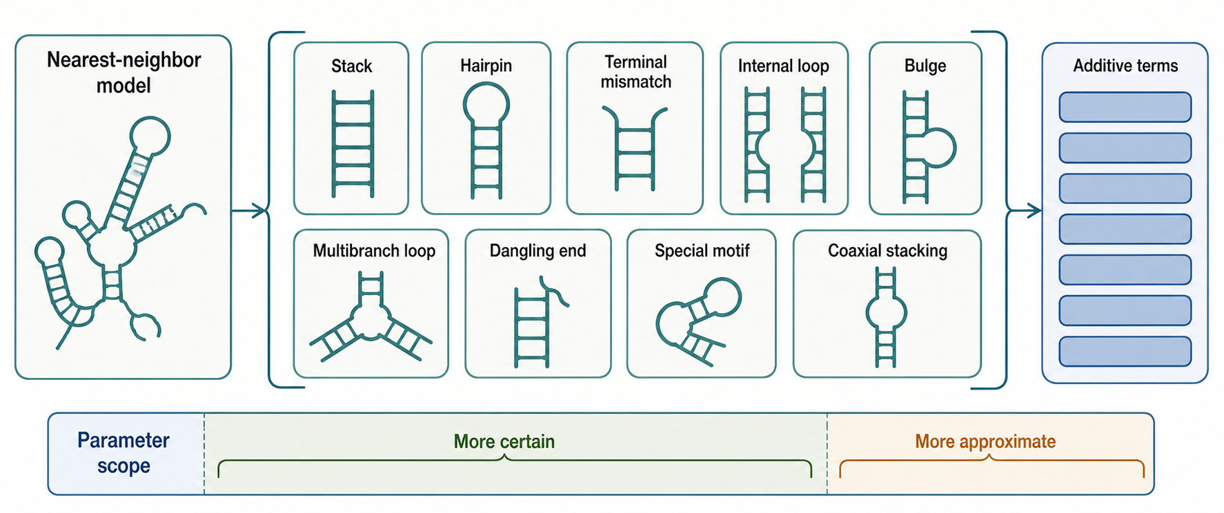
Figure 60.3. Energy Terms in a Nearest-Neighbor Folding Model. Nearest-neighbor folding models approximate total free energy by adding terms for stacked base pairs, loop initiation, terminal mismatches, dangling ends, internal loops, bulges, multibranch loops, special motifs, and sometimes coaxial stacking. The additivity is useful and interpretable, but every term has a parameter scope defined by the experimental data used to derive it, and terms for multibranch loops and coaxial stacking are more approximate than helix-stacking terms.
Thermodynamic parameters are usually derived from measurements on short oligonucleotides under defined buffer, salt, and temperature conditions. Optical melting experiments measure how absorbance changes as duplexes or hairpins unfold with temperature. Fitting those curves yields enthalpy, entropy, and free-energy estimates for motifs. Those motif values are then used additively in folding algorithms. This is a major abstraction. A parameter measured in a short RNA duplex is applied inside longer RNAs, in junctions, or near other motifs. The approximation works well enough to be valuable, but it is less reliable when local motifs are coupled to tertiary structure, proteins, modified bases, or long-range electrostatics.
Modified nucleotides illustrate both the strength and the limitation of parameterization. Natural and engineered RNAs often contain N6-methyladenosine, pseudouridine, 2′-O-methylated nucleotides, inosine, synthetic substitutions, labels, or therapeutic chemistry. Standard RNA folding parameters assume the four canonical bases unless special parameters are supplied. Kierzek and colleagues showed that secondary-structure prediction can be extended for sequences including N6-methyladenosine, and Richardson and Znosko measured parameters for 7-deaza-adenosine-uridine pairs. These studies do not mean that all modified RNAs can now be predicted accurately. They show the path: measure the thermodynamics of the modified motif, encode the parameter, and state the scope of validity.
Nearest-neighbor prediction also depends on conditions. Temperature changes the balance of enthalpy and entropy. Magnesium can stabilize compact folds and tertiary contacts not represented by a simple secondary-structure model. Monovalent salt screens electrostatic repulsion. Ligands and proteins can selectively stabilize folds. Crowding and co-transcriptional emergence can change accessible states. A computed MFE at a default temperature is therefore not a universal property of the sequence. It is the optimum under the program’s condition assumptions.
The additive model has a useful pedagogical consequence. Users can inspect why a structure is predicted to be stable. A long GC-rich helix contributes favorable stacking terms. A small hairpin loop may be costly unless it has stabilizing sequence features. A large asymmetric internal loop can destabilize a stem. A multibranch junction may be penalized enough that an alternative two-hairpin structure wins. This energy decomposition turns folding prediction into testable reasoning. If a predicted helix depends on a few weak terminal pairs, mutating or constraining those pairs may change the fold. If two structures differ mainly in multiloop terms, the prediction may be sensitive to poorly known parameters.
60.4. Constraints, dangling ends, loops, and coaxial stacking
Constraints let users inject external knowledge into a folding calculation. A hard constraint can require a known pair, prohibit a pair inconsistent with an experiment, or force a nucleotide to be unpaired because it must bind a protein or participate in a catalytic site. A soft constraint adjusts the energy function without making alternatives impossible. For example, a nucleotide that is highly reactive in a SHAPE experiment can be penalized when predicted paired, but the algorithm may still pair it if other evidence in the model strongly favors that structure. Chapter 63 gives full treatment to probing-constrained modeling; here the important point is that constraints change the formal problem being solved.
Constraints are powerful because pure thermodynamics is often underdetermined. A riboswitch aptamer may be known from biochemical evidence to require a helix that the unconstrained model misses. A viral RNA pseudoknot may have a crossing pair set that a standard non-pseudoknotted algorithm cannot represent, but a user may still constrain local stems around the pseudoknot. A designed guide RNA may have regions that must remain accessible for target binding. In these cases, constraints can convert biological knowledge into a better computational hypothesis.
Constraints can also mislead. A chemical-probing protection can result from protein binding, tertiary packing, RNA modification, poor reagent access, or low coverage, not only Watson-Crick pairing. Forcing every protected nucleotide into a helix can create a plausible but wrong model. A covariation-supported pair in one homologous family may not apply to a divergent sequence with a different regulatory state. A required pair from an old drawing may perpetuate an obsolete model. Constraint files should therefore be documented with evidence type, condition, and uncertainty.
Dangling ends are unpaired nucleotides adjacent to a helix terminus that can stack on the helix and change stability. They matter most at helix ends and loop boundaries. Different programs and parameter settings can treat dangles differently: use no dangle contributions, use one side, allow both sides under restrictions, or optimize dangles during folding. This can change predicted energies and sometimes structures, especially for short RNAs where end effects are large. A small engineered hairpin may look more or less stable depending on dangle treatment.
Loops are where much of the biological and algorithmic complexity resides. A hairpin loop closes a stem with a single-stranded loop. A bulge loop has unpaired nucleotides on one side of a helix. An internal loop has unpaired nucleotides on both sides. A multibranch loop joins three or more helices. These categories are simplified two-dimensional descriptions, but they capture many energetic costs. Small stable tetraloops, asymmetric internal loops, and junctions with coaxial stacking can dominate folding outcomes.
Coaxial stacking occurs when two helices align end-to-end so that base stacking continues across a junction. This is a secondary-structure-adjacent approximation of a three-dimensional arrangement. It is especially relevant in multibranch loops, ribozymes, riboswitches, and structured viral RNAs where junction geometry determines global architecture. Including coaxial stacking can improve some predictions but also increases model complexity. Courtney and colleagues’ sparse folding work including coaxial stacking reflects continued interest in modeling this feature efficiently. The cautious interpretation is that coaxial stacking is real and often important, but predicting it from sequence alone remains more uncertain than predicting a simple helix.
The deepest boundary case is the pseudoknot. A pseudoknot can include ordinary stems and loops locally, but the crossing topology violates the nesting assumptions of standard dynamic programming. Many biologically central RNAs use pseudoknots, including telomerase RNA regions, viral frameshift signals, ribozymes, and ribosomal RNA elements. A Zuker-style non-pseudoknotted prediction may still identify local stems in those RNAs, but it cannot fully represent the pseudoknotted architecture. Hollar and colleagues review this algorithmic and biological boundary.
60.5. Benchmarking, accuracy, and failure modes
Benchmarking asks whether predicted structures match reference structures. The usual comparison treats a secondary structure as a set of base pairs. Sensitivity measures the fraction of reference base pairs recovered by the prediction. Positive predictive value measures the fraction of predicted base pairs that appear in the reference. The F1 score combines the two. These metrics are useful because they are explicit, but they also reduce RNA structure to a pair list and depend heavily on the quality and relevance of the reference.
A reference structure may come from crystallography, cryo-EM, NMR, comparative covariation, targeted biochemical mapping, or expert annotation. None is perfect. A high-resolution structure may come from a truncated construct, a bound protein, a ligand, or nonphysiological buffer. A comparative structure may represent a conserved family fold rather than a specific cellular state. A chemical-probing-informed model may encode reactivity assumptions. A database annotation may persist after newer evidence complicates it. Therefore a benchmark result should state what reference was used and why it is appropriate for the claim.
Thermodynamic MFE algorithms tend to work best for shorter, well-behaved RNAs whose native folds are dominated by local secondary-structure energetics and whose motifs are covered by the parameter set. Transfer RNA cloverleafs, many small hairpins, some riboswitch domains, and designed small RNAs can be reasonably tractable, though even these have tertiary contacts and modifications that matter. Accuracy tends to decline for long RNAs, RNAs with multiple domains, RNAs whose folding is co-transcriptional, RNAs with extensive protein binding, RNAs with pseudoknots, and RNAs where small energy differences separate alternative states.
One common failure mode is overconfidence in a single MFE drawing. If the MFE structure and several alternatives lie close in energy, the exact drawing may be unstable to small parameter changes or sequence edits. A second failure mode is long-range false pairing. In long RNAs, an energetically favorable helix can be predicted between regions that never meet in the biological context because proteins, ribosomes, transcription timing, or domain organization prevent the interaction. A third failure mode is missing functional accessibility. A translation-initiation region might be predicted paired, but ribosome scanning, helicases, or RNA-binding proteins can open it. A fourth failure mode is treating absence of a predicted structure as absence of function. Some regulatory RNAs act through transient structures, protein-assisted folding, or sequence motifs that thermodynamic MFE prediction is not designed to detect.
Machine-learning and hybrid methods have changed the benchmark landscape but have not made thermodynamic reasoning obsolete. Deep-learning methods can learn patterns from known structures and sometimes outperform pure thermodynamic models on benchmark sets. Sato and colleagues integrated deep learning with thermodynamic information, and UFold illustrated a fast deep-learning approach to secondary-structure prediction. Reviews emphasize both progress and persistent challenges: training-set bias, structure redundancy, uncertainty calibration, modified nucleotides, pseudoknots, and generalization to unusual RNA classes remain difficult. A model can win a benchmark and still fail for a newly designed therapeutic RNA or a viral element outside its training distribution.
Benchmarking should also include negative controls and reproducibility checks. A useful pipeline records the input sequence, software, version, command, parameter set, constraints, temperature, and output. It tests whether small edits or alternative parameter sets change conclusions. It compares local and global folding when the biological question is local. It avoids cherry-picking the one structure that matches a favored model. For publication-quality interpretation, prediction should be paired with experimental or comparative evidence whenever the claim is mechanistic.
The supplied bibliography for this chapter contains strong review and method anchors for folding algorithms, thermodynamic integration, modified-base parameters, multiloop modeling, coaxial stacking, and pseudoknots. Its benchmarking subsection also contains several off-topic automated references from unrelated RNA computational domains. Those off-topic references should not be used as direct evidence for secondary-structure benchmark accuracy. Final-reference expansion: add verified direct benchmark sources for RNA secondary-structure prediction accuracy, dataset construction, and package comparison before final publication.
60.6. Software ecosystems and reproducible prediction
RNA secondary-structure prediction is implemented in a software ecosystem rather than a single canonical program. Widely used thermodynamic lineages include mfold, RNAstructure, and the ViennaRNA package, alongside many specialized tools for local folding, constrained folding, design, pseudoknots, comparative folding, probing integration, and machine learning. Final-reference expansion: add verified package-specific citations for mfold, ViennaRNA, RNAstructure, CONTRAfold, LinearFold, and other commonly used software after citation-key curation. The practical point for this chapter is that software choice affects not only convenience but also scientific output.
Programs can differ in parameter updates, dangle models, treatment of lonely pairs, maximum internal-loop size, multiloop scoring, coaxial stacking, pseudoknot support, constraint syntax, output format, and default temperature. They can also differ in whether they fold DNA, RNA, or mixed modified sequences; whether they expose partition functions; whether they support SHAPE pseudoenergies; and whether they report suboptimal structures in comparable ways. A dot-bracket string from one program is therefore not automatically interchangeable with a dot-bracket string from another.
Reproducible prediction begins with input hygiene. The sequence should be stated in 5′ to 3′ orientation, with clear handling of U versus T, ambiguous bases, lower-case masking, modified residues, adapters, poly(A) tails, and transcript boundaries. Folding a complete transcript, a mature processed RNA, a UTR fragment, or a sliding window can answer different questions. For a 5′ UTR, including the coding sequence may change predicted structure around the start codon. For a riboswitch, including or excluding the expression platform can switch the dominant fold. For a guide RNA, trimming constant scaffold regions may destroy the structure actually used in the ribonucleoprotein.
A reproducible methods statement should include at least the software name and version, parameter set, temperature, input sequence or accession and coordinates, command-line options, constraints, and post-processing choices. If suboptimal structures are reported, the energy window or sampling method should be stated. If a structure was selected from many outputs because it matched an experiment, that selection should be described transparently. If a default was used, the default should still be documented because software defaults can change.
Software ecosystems now include thermodynamic, learned, and hybrid methods. Chapter-level reviews compare many tools and describe a field moving toward integrated prediction, but the core thermodynamic model remains valuable because it is interpretable, parameterized, and fast. Geng and colleagues’ recent work on predicting cellular RNA activity from conformational ensembles illustrates a broader trend: the output of folding calculations is increasingly connected to functional activity rather than treated as an isolated drawing. The strongest future pipelines will likely combine thermodynamic interpretability, learned pattern recognition, experimental constraints, and explicit uncertainty.
Experimental Foundations and Evidence
Thermodynamic RNA folding rests on experimental foundations, even when users encounter it as software. The parameters originate from measurements on defined molecules. The structures used for benchmarking originate from structural biology, biochemical mapping, and comparative analysis. The failure modes are revealed when predictions are tested against mutational rescue, ligand binding, enzymatic activity, translation, splicing, RNA decay, or viral replication. This evidence chain should remain visible.
A predicted helix becomes more credible when compensatory mutations support base pairing. A predicted riboswitch fold becomes more credible when ligand binding changes chemical probing, transcription termination, and gene expression in the expected direction. A predicted viral RNA element becomes more credible when disrupting the structure impairs replication and restoring pairing rescues it. A predicted therapeutic RNA structure becomes more credible when it improves target engagement, stability, or translation under relevant assay conditions. Prediction alone can prioritize experiments, but it rarely completes the causal argument.
Box 60.2. Evidence Ladder for a Predicted Helix
- Prediction only: lowest credibility; establishes a structural hypothesis from sequence alone.
- Prediction plus conservation: homologous sequences fold similarly, supporting the motif but not function in a specific context.
- Prediction plus chemical probing: reactivity patterns consistent with the predicted pairing increase plausibility.
- Disruptive mutation: substitutions that break the predicted helix reduce biological activity, implicating the structure.
- Compensatory rescue: a second mutation restoring base pairing restores activity, providing strong support for the helix.
- Structural observation: crystallographic, cryo-EM, or NMR data confirm the base-pairing arrangement directly.
- Functional mechanism: the structural element is shown to participate in a specific molecular step such as ligand binding, catalysis, or regulatory switching.
Biological Contexts Across RNA Classes
Thermodynamic prediction is most straightforward for RNAs whose functional structure is primarily an intramolecular secondary structure. Many small regulatory elements, aptamers, and engineered hairpins fit this description partly. It is less straightforward for large cellular RNAs that fold while being transcribed, translated, processed, bound by proteins, modified, and degraded. Messenger RNAs are especially context dependent: local structures can affect splicing, localization, translation, and decay, but the relevant structure may be the structure in an RNP, not the naked RNA MFE.
Stable RNAs such as tRNAs and rRNAs show another boundary. Their secondary structures are conserved and often predictable in outline, but their biological forms depend on modifications, tertiary contacts, ribosomal proteins, processing, and assembly. Viral RNAs often contain compact structured elements and long-range interactions, but many viral elements include pseudoknots or alternative conformations. Therapeutic and synthetic RNAs can be designed with folding software, yet modified nucleotides, delivery formulation, innate immune sensing, and protein binding can change the cellular outcome.
The chapter’s practical rule is to match prediction scale to biology. Use MFE folding to reason about a local hairpin, a competing riboswitch helix, a designed guide scaffold, or a candidate regulatory element. Use ensemble, probing-constrained, comparative, or tertiary approaches when the claim concerns population behavior, in-cell structure, homologous conservation, or three-dimensional architecture.
Technology, Computational, Clinical, and Engineering Links
Thermodynamic secondary-structure prediction is embedded in RNA technology. It helps design primers, probes, guide RNAs, aptamers, ribozymes, siRNAs, mRNA UTRs, riboswitches, and RNA nanostructures. It helps avoid unintended self-complementarity, estimate accessibility, and compare candidate sequences. In therapeutic mRNA design, local structure can affect translation, stability, innate immune sensing, manufacturing, and analytical behavior, although no single MFE prediction captures all of these effects. In oligonucleotide therapeutics, duplex stability and target accessibility matter, but chemical modifications and protein binding require parameters or empirical testing.
Engineering use places extra weight on reproducibility. A design pipeline may screen thousands of sequences, so silent changes in software version or parameters can alter ranked candidates. A clinical or manufacturing setting needs auditable methods, not only a pleasing predicted drawing. When prediction influences a therapeutic or diagnostic design, the method should be treated as part of the design history: input sequence, constraints, outputs, parameter set, and decision rule should be preserved.
Recent Consensus
Recent consensus is that thermodynamic MFE prediction remains a foundational, interpretable, and fast baseline for RNA secondary structure, but it should not be treated as a complete cellular folding model. Dynamic programming and nearest-neighbor parameters are still central for single-sequence folding. Parameter extensions for modified nucleotides and specialized motifs are valuable but necessarily incomplete. Multiloop and coaxial-stacking treatment remains an active area where additional complexity must be justified by performance and parameter support.
The software landscape is now plural. Thermodynamic, machine-learning, hybrid, comparative, and experimentally constrained methods answer overlapping but distinct questions. A modern workflow often begins with MFE prediction, checks suboptimal alternatives, examines ensemble uncertainty, incorporates probing or comparative constraints when available, and validates biological claims experimentally. The field’s center of gravity has shifted from “What is the one structure?” to “Which structures are plausible under which evidence and conditions?”
Open Questions, Controversies, Deprecated Models, and Common Misconceptions
Open questions:
- How much physical detail should be added to thermodynamic models? More terms can represent more biology, but every term needs parameters. A complex multiloop or coaxial-stacking model can overfit sparse data. Ward and colleagues’ conclusion that a simpler multiloop model performed best in their analysis is a useful caution against assuming that model elaboration is automatically progress.
- How can researchers handle modified and chemically engineered RNAs at scale? Individual modifications can be parameterized, as shown for N6-methyladenosine and 7-deaza-adenosine contexts. But the space of modifications, combinations, backbone chemistries, and formulation conditions is far larger than the measured parameter space. Prediction for modified therapeutic RNAs should therefore be labeled according to what was parameterized and what was approximated.
Controversies:
- Benchmark interpretation remains controversial. A method can improve an aggregate score while performing poorly on the RNA class a user cares about. Training-set overlap can inflate machine-learning performance. Reference structures can be biased toward stable, crystallizable, conserved, or short RNAs. Long RNAs may be judged against incomplete annotations. The best benchmark is not the largest table; it is the benchmark whose reference structures, molecule classes, and evaluation metrics match the intended use.
Common misconceptions:
- “The MFE structure is not necessarily the native structure.” A low computed free energy is not evidence of function. A predicted unstructured region is not necessarily unstructured in a cell. A missing pseudoknot in a standard fold is not evidence that a pseudoknot is absent.
- “A SHAPE-constrained prediction is not direct structure determination.” A deep-learning prediction is not automatically more reliable than a thermodynamic prediction outside its training domain. A beautiful RNA drawing is a hypothesis until evidence supports it.