Chapter 146. Systems RNA Biology, Multi-Omics Integration, Quantitative Models, and Organism-Scale Regulation
Scope Note
This chapter treats RNA regulation as an integrated system rather than a sequence of isolated molecular events. It connects omics layers, kinetic models, network dynamics, evolutionary comparison, artificial intelligence, causal inference, and validation design.
Executive Summary
Systems RNA biology asks how RNA-centered molecular events combine to produce cellular behavior. A single RNA molecule has a life history: the RNA is transcribed, capped or otherwise end-processed, spliced or cleaved when relevant, chemically modified, assembled with proteins, exported or retained, transported or localized, translated or used as a noncoding regulator, stored, surveilled, and degraded. Each step can be measured imperfectly by a different assay. Transcriptomics reports accumulated RNA molecules; nascent RNA assays report production and early processing; translatomics reports ribosome engagement; proteomics reports protein output; epigenomic assays report chromatin state and regulatory potential; metabolomics reports biochemical state; perturbation screens report responses to intervention; and spatial assays report where molecular states occur in tissues. Integration becomes biological only when these layers are mapped to the molecular processes they observe and to the time scales on which those processes change.
Quantitative models provide the grammar for integration. A steady-state RNA abundance can increase because synthesis rises, decay falls, processing becomes more efficient, export changes, cell composition shifts, or a measurement artifact changes. Without time, perturbation, nascent-RNA data, or compartment information, these alternatives can be mathematically indistinguishable. Kinetic models, stochastic birth-death models, state-space models, Bayesian hierarchical models, and machine-learning predictors each make assumptions about what is measured and what must be inferred. Good models expose their assumptions, report uncertainty, and identify which parameters are estimable under the experimental design.
RNA systems are also networks. RNA-binding proteins, small RNAs, miRNAs, splicing factors, RNA decay enzymes, translation factors, polymerases, chromatin regulators, metabolites, and signaling pathways form feedback and feed-forward architectures. These architectures can buffer noise, generate thresholds, tune pulse duration, create memory, or drive state transitions, but a network diagram alone does not establish dynamic behavior. Rates, delays, molecular saturation, compartmentalization, and energy or resource constraints decide whether a motif stabilizes a system, amplifies a fluctuation, or oscillates.
Evolutionary systems biology extends these questions across species and lineages. Comparative transcriptomics can identify conserved RNA programs, lineage-specific innovations, regulatory rewiring, and conserved outputs produced by different molecular mechanisms. Orthology, cell-type matching, annotation quality, tissue composition, phylogenetic relatedness, and batch structure must be handled before expression differences are interpreted as biological evolution. Conservation can occur at the level of RNA sequence, structure, target, expression pattern, dynamic response, or network function; these layers often evolve at different rates.
Artificial intelligence and causal inference are useful only when their claims are kept separate. AI models can learn representations, prioritize regulatory motifs, predict perturbation responses, impute missing modalities, propose candidate RNA functions, and assemble organism-scale knowledge graphs. Causal inference asks a stricter question: what would change if a specific RNA, regulator, sequence element, cell state, or environmental input were intervened on? Observational association, prediction accuracy, and feature importance do not answer that question by themselves. Perturbation screens, rescue experiments, epistasis, temporal ordering, independent validation, and biochemical mechanism remain central.
The main limitation of systems RNA biology is not lack of data; it is mismatched data. Datasets may be generated in different batches, tissues, species, cell states, time points, platforms, or annotation versions. Some modalities are missing because they are expensive, destructive, sparse, or incompatible with the same cells. Benchmarks can leak information through shared sequences, duplicated perturbations, reused annotations, or target-derived features. Reliable systems RNA biology therefore depends on explicit model assumptions, careful benchmark design, orthogonal validation, and a culture of distinguishing established mechanism from attractive integrated narratives.
Concept Inventory
- Systems RNA biology: RNA production, processing, localization, translation, decay, and regulatory effects studied as coupled cellular, tissue, organismal, and evolutionary systems.
- Multi-omics integration: joint analysis of molecular layers such as RNA, chromatin, ribosome occupancy, protein, metabolite, spatial, and perturbation data, with explicit handling of scale, noise, time, and alignment.
- Translatomics: transcriptome-wide measurement of translation-related states, especially ribosome occupancy, polysome association, nascent peptide production, or translation efficiency.
- Quantitative model: a mathematical or computational representation of biological variables, transitions, rates, observations, assumptions, and uncertainty.
- Identifiability: the degree to which data and assumptions can determine a model parameter, such as synthesis rate or decay rate.
- Network motif: a recurring regulatory wiring pattern, including negative feedback, positive feedback, feed-forward control, buffering, mutual antagonism, and delayed activation.
- Causal inference: estimation of what would change under a defined intervention rather than what variables merely correlate.
- Organism-scale RNA knowledge graph: a structured representation linking RNA entities, regulators, contexts, perturbations, evidence, and citations with explicit edge meanings.
What to Know Before Reading This Chapter
The chapter assumes familiarity with the central flow of gene expression: DNA can be transcribed into RNA, RNA can be processed into mature forms, and some RNAs are translated into proteins. It also assumes that the reader knows that many RNAs are noncoding and that many regulatory steps occur after transcription. Earlier chapters explain the molecular details of capping, splicing, polyadenylation, export, decay, translation, RNA localization, RNA-binding proteins, small RNAs, single-cell assays, ribosome profiling, perturbation screens, RNA informatics, and evidence standards. This chapter uses those mechanisms as components of larger systems.
A useful running example is a stress-response mRNA in a mammalian immune cell. A signaling pathway activates transcription factors, chromatin becomes more accessible near the gene, nascent RNA synthesis increases, splicing and 3′ end formation occur, the mRNA exits the nucleus, RNA-binding proteins and miRNAs tune stability and translation, ribosomes produce protein, metabolites change as the cell shifts state, and the protein feeds back on signaling. A bulk RNA-seq experiment sees only one projection of this story: the number of RNA molecules accumulated at a sampling time. A systems approach asks which steps changed, how the steps interact, how the cell population is structured, and which perturbation would distinguish competing mechanisms.
The most important caution is that integrated data are not automatically integrated evidence. If RNA abundance, protein abundance, and chromatin accessibility all change in the same condition, the shared change may reflect a single causal pathway, a shift in cell-type composition, a batch effect, or an unmeasured environmental variable. Systems RNA biology becomes strong when it connects measurement to mechanism, mechanism to intervention, and intervention to validation.
146.1. Integrating Transcriptomics, Translatomics, Proteomics, Epigenomics, Metabolomics, Perturbation Screens, and Spatial Data
Multi-omics integration begins with a simple discipline: define what each measurement directly observes. Transcriptomics measures RNA abundance, sequence, isoform structure, or RNA-derived counts. A mature RNA-seq count is usually closer to accumulated RNA abundance than to transcription rate. Nascent RNA assays, metabolic labeling, and chromatin-associated RNA assays move closer to production and early processing. Long-read RNA sequencing can connect exons, transcript ends, and isoforms within single molecules. Single-cell RNA-seq measures sparse transcript counts in individual cells or nuclei, often with strong dropout and capture bias. Spatial transcriptomics adds tissue position, but most spatial methods trade molecular sensitivity, resolution, or transcript coverage for location.
Translatomics measures translation-related states. Ribosome profiling reports ribosome-protected fragments and can reveal translated open reading frames, upstream open reading frames, codon-level pauses, and condition-specific changes in ribosome occupancy. Polysome profiling separates RNAs by ribosome association and is less precise at nucleotide resolution but can be robust for broad translation-state changes. These assays bridge RNA and protein output, yet they do not eliminate the need for proteomics. A transcript can be heavily ribosome-associated while producing an unstable protein, a paused nascent chain, or a protein whose abundance is dominated by degradation. Conversely, a stable protein can persist long after its mRNA declines.
Proteomics measures proteins, usually by mass spectrometry or antibody-based methods. The proteome is downstream of translation, folding, localization, modification, and degradation. Integration of RNA-seq and proteomics can identify transcripts whose protein output is concordant with RNA abundance, transcripts under translational control, and proteins whose abundance is controlled primarily by degradation or complex assembly. Interpretation must respect dynamic delay. If an mRNA rises at 30 minutes and its protein rises at 4 hours, a simultaneous snapshot may look discordant even when the RNA causes the protein change.
Epigenomics is used here as a practical shorthand for genome-associated regulatory measurements, including chromatin accessibility, transcription-factor occupancy, histone modifications, DNA methylation, three-dimensional genome contacts, and chromatin-associated RNA. These assays do not measure RNA regulation directly, but they can constrain models of RNA production. For example, increased accessibility at an enhancer and increased nascent transcription at a target gene support a production-side mechanism more strongly than mature RNA abundance alone. Boundary cases matter. Accessible chromatin is not proof of transcription. A histone mark is not proof of enhancer function. A chromatin contact is not proof that an enhancer regulates a gene unless perturbation or additional evidence supports the link.
Metabolomics measures small molecules and biochemical state. Metabolites can affect RNA biology through nucleotide availability, energy charge, methyl-donor pools, redox state, stress signaling, riboswitch ligands, RNA modification substrates, and translation or decay pathways. In bacteria, a metabolite-binding riboswitch can directly change transcription termination or translation initiation. In eukaryotic cells, metabolic state can alter RNA modification, translation initiation, stress granule formation, and mRNA decay indirectly through signaling and enzyme activity. Metabolomics is often less directly mappable to single RNA molecules than transcriptomics or ribosome profiling, but it can explain why RNA regulatory programs change with growth, stress, differentiation, or immune activation.
Perturbation screens add intervention. CRISPR knockout, CRISPR interference, CRISPR activation, RNA interference, antisense oligonucleotides, drug treatments, reporter libraries, saturation mutagenesis, and environmental perturbations can test whether a candidate regulator changes an RNA outcome. Perturb-seq-like designs combine perturbations with single-cell RNA readouts. Reporter libraries can test thousands of UTRs, codon variants, splice elements, or RNA-binding protein motifs. These methods are powerful because they move beyond observation, but they introduce their own artifacts: incomplete perturbation, off-target effects, variable guide efficiency, toxicity, compensation, cell-cycle shifts, and selection against strong phenotypes.
Spatial data anchor RNA systems in tissue architecture. A neuron, an epithelial cell, an immune cell, and a stromal cell can express related RNA programs but use them in different spatial contexts. RNA localization within a cell also matters: dendritic mRNAs, endoplasmic-reticulum-associated mRNAs, mitochondrial-proximal mRNAs, stress-granule-associated RNAs, and nuclear-retained RNAs can have distinct fates even when total abundance is unchanged. Tissue spatial methods and subcellular localization methods therefore answer different questions. Tissue maps ask where cell states and RNA programs occur relative to anatomy. Subcellular methods ask where individual RNA molecules are transported, anchored, translated, stored, or degraded.
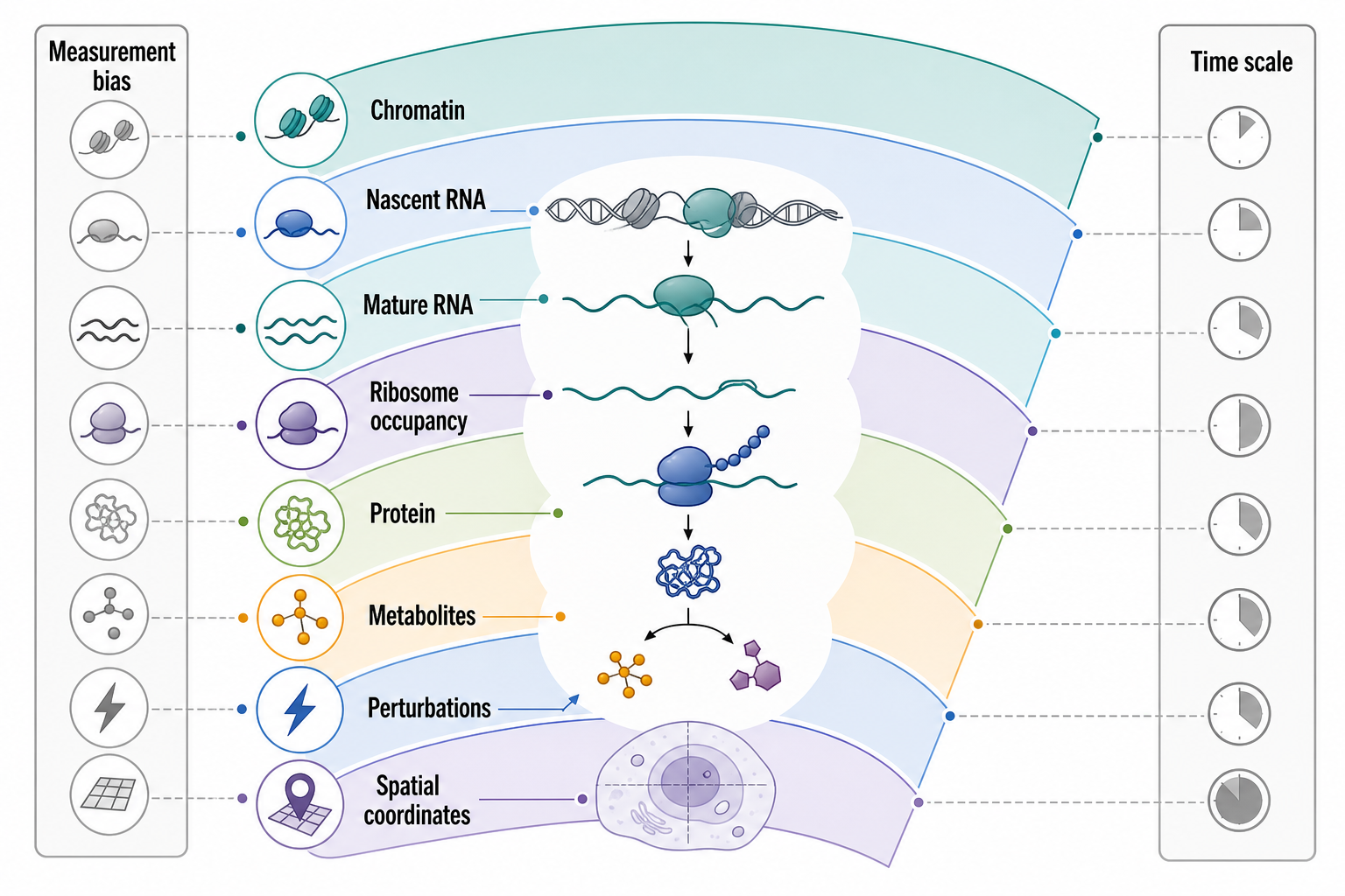
Figure 146.1. Multi-Omics Layers Around an RNA-Centered Gene Expression Program. A systems RNA biology experiment aligns measurements with the molecular steps they can observe. Chromatin and nascent-RNA assays report regulatory potential and RNA production, bulk or single-cell RNA-seq reports accumulated transcript molecules, Ribo-seq and related assays report ribosome engagement, proteomics reports protein output, metabolomics reports biochemical state, and spatial assays report where these states occur in tissue. Integration is strongest when each layer is modeled with its measurement bias and time scale.
The practical challenge is alignment. Bulk RNA-seq and proteomics may be performed on the same homogenized sample, but the measured tissue can contain changing proportions of cell types. Single-cell RNA-seq and single-cell chromatin accessibility can measure similar cells but often not the same molecule or the same physical cell unless a paired multiome assay is used. Spatial transcriptomics may measure tissue position but lack full isoform resolution. Proteomics and metabolomics often require more material than single-cell RNA assays and may be performed on matched but not identical samples. A computational integration method must therefore decide whether it is aligning samples, cells, neighborhoods, time points, perturbations, genes, pathways, or latent states.
Box 146.1. Alignment Is a Claim, Not a Merge
Alignment Is a Claim, Not a Merge
A multi-omics matrix becomes meaningful only after the analyst states what is being aligned. Same-sample evidence means two layers were measured from the same biological specimen, such as RNA-seq and proteomics from one tissue homogenate. Same-cell evidence is stronger but rarer, because many assays destroy the cell or require incompatible preparation. Matched-sample evidence uses paired donors, regions, time points, or cell states, but the correspondence is inferred rather than direct. Reference-based evidence maps a new dataset onto an external atlas; it is useful for annotation but vulnerable to differences in species, disease, platform, or developmental stage. Imputed evidence fills missing values from a model and should be treated as prediction, not measurement. Before interpreting an integrated result, ask: aligned by what unit, observed in which layer, and validated by what independent assay?
An RNA-centered integration workflow begins with a biological question. If the question is whether a stimulus increases transcription of an mRNA, nascent RNA and chromatin data are central, while proteomics is downstream. If the question is whether an mRNA is translationally repressed, ribosome profiling, polysome association, reporter assays, and proteomics become central. If the question is whether a noncoding RNA alters chromatin, RNA perturbation plus chromatin readouts and rescue are needed. If the question is whether a disease-associated variant changes splicing, long-read RNA sequencing, splice-junction analysis, minigene reporters, and allele-specific assays may be more informative than total gene counts.
Table 146.1. Modalities, Molecular Questions, and RNA-Centered Outputs. Transcriptomic, translatomic, proteomic, metabolomic, epigenomic, spatial, and perturbational layers measure different RNA-system outputs; integration should preserve each layer’s assay limits and regulatory timescale.
| Modality or data layer | RNA-centered output | Evidence or caveat |
|---|---|---|
| Mature RNA-seq | Estimates accumulated RNA abundance, splice-junction usage, and gene- or transcript-level output after synthesis, processing, export, localization, and decay have already acted. | Mature RNA abundance cannot by itself distinguish increased synthesis from decreased decay, altered cell composition, or mapping and annotation effects. |
| Nascent RNA and metabolic labeling | Constrains transcriptional output, early processing, and turnover timing more directly than steady-state RNA-seq. | Labeling efficiency, time resolution, nucleotide metabolism, and incomplete separation of nascent from mature pools can affect inferred rates. |
| Long-read RNA sequencing | Links exons, transcript ends, isoforms, retained introns, fusion transcripts, and allele-specific transcript structures within single molecules. | Lower depth, platform-specific errors, size selection, and library preparation bias can make rare isoforms or quantitative comparisons uncertain. |
| Single-cell or single-nucleus RNA-seq | Resolves cell-state heterogeneity, cell composition, and transcriptome-level responses in individual cells or nuclei. | Sparse capture, dissociation stress, dropout, cell-cycle effects, and nucleus-versus-cell differences can mimic biological structure. |
| Spatial and subcellular RNA assays | Places RNA programs in tissue neighborhoods or within cellular compartments such as dendrites, endoplasmic-reticulum-associated regions, granules, or nuclei. | Tissue spatial maps and subcellular localization assays answer different questions; resolution, segmentation, and sensitivity limit interpretation. |
| Ribosome profiling and polysome profiling | Reports ribosome engagement, translated open reading frames, upstream open reading frames, ribosome pauses, and broad translation-state shifts. | Ribosome occupancy is not protein abundance; initiation, elongation, pausing, ribosome recycling, and protein degradation must be considered. |
| Proteomics | Measures protein output after translation, folding, localization, modification, complex assembly, and degradation. | Protein stability and mass-spectrometry detectability can uncouple protein abundance from RNA abundance or ribosome loading. |
| Chromatin and epigenomic assays | Constrains production-side hypotheses through accessibility, transcription-factor occupancy, histone marks, DNA methylation, contacts, and chromatin-associated RNA. | Accessible chromatin, a histone mark, or a contact is regulatory potential rather than proof of enhancer function without perturbation or convergent evidence. |
| Metabolomics | Reports biochemical state that can affect nucleotide supply, energy charge, methyl-donor pools, riboswitch ligands, RNA modification, translation, and decay pathways. | Metabolites are often pathway-level rather than RNA-specific readouts, and annotation, ion suppression, and batch effects can limit mechanistic assignment. |
| Perturbation screens and reporter libraries | Tests whether candidate regulators, RNA elements, splice sites, UTRs, codon variants, or environmental inputs change RNA-centered outcomes. | Off-target effects, incomplete perturbation, toxicity, guide efficiency, compensation, and selection against strong phenotypes must be modeled or controlled. |
The evidence basis of multi-omics integration is strongest when orthogonal measurements converge on the same mechanism while retaining their independence. For example, a model of increased mRNA production is strengthened by increased nascent RNA, promoter or enhancer activation, time-ordered mature RNA increase, and loss of the response after perturbing the upstream transcription factor. A model of increased translation is strengthened by unchanged mRNA abundance, increased ribosome loading, increased nascent peptide or protein production, reporter dependence on a UTR or coding feature, and loss of the response after perturbing the relevant translation regulator. A model of altered RNA decay is strengthened by pulse-chase labeling, decay after transcriptional shutoff, changes in deadenylation or decapping factors, and rescue by mutating the relevant cis-element.
The boundary case is an integrated story that is really a correlated atlas. Atlases are valuable because they describe cell states, tissues, developmental trajectories, and disease contexts. They become mechanistic only when they identify which variables are causes, which are consequences, and which are markers. The handoff to the next section is therefore natural: integration needs quantitative models that connect measurements to rate processes.
146.2. Quantitative Models of RNA Production, Processing, Export, Localization, Translation, and Decay
A quantitative model of RNA regulation converts a verbal mechanism into variables, transitions, rates, and observations. The simplest useful model of an mRNA has two rates: synthesis and degradation. If synthesis occurs at rate k_s and degradation occurs at rate k_d, the expected abundance at steady state is proportional to k_s / k_d. This equation teaches a central lesson: an observed abundance is a ratio of processes. A twofold increase in RNA abundance could come from increased synthesis, decreased degradation, or both. Without additional data, the cause is not identifiable.
Box 146.2. Rate Claims Need Rate Evidence
Rate Claims Need Rate Evidence
When an mRNA changes abundance, the first safe statement is descriptive: more or fewer RNA molecules were observed under the specified assay and normalization. A rate claim is stronger. “Transcription increased” requires evidence closer to synthesis, such as nascent transcription, metabolic labeling, promoter-proximal polymerase signal with appropriate controls, or an early time course. “Decay slowed” requires pulse-chase, transcriptional shutoff, direct half-life estimation, deadenylation or decapping evidence, or a perturbation of a decay pathway. “Export changed” requires nuclear-cytoplasmic separation, imaging, or compartment-specific sequencing. “Translation changed” requires ribosome, nascent-chain, reporter, or proteomic evidence. A model may fit multiple rate combinations to the same RNA-seq endpoint. The pedagogical rule is: name the observed quantity first, then state which extra measurement converts that observation into a kinetic claim.
Real RNA life histories contain more states. A eukaryotic pre-mRNA is transcribed by RNA polymerase II, capped, spliced, cleaved, polyadenylated, packaged into a messenger ribonucleoprotein particle, exported through the nuclear pore, localized in the cytoplasm, translated, stored, surveilled, deadenylated, decapped, and degraded. A bacterial mRNA may be transcribed, fold co-transcriptionally, bind ribosomes while still being transcribed, interact with small RNAs, and be degraded by ribonucleases while translation is ongoing. A long noncoding RNA may be retained in the nucleus, processed inefficiently, bind chromatin or proteins, and decay rapidly. A miRNA is transcribed, processed by Drosha and Dicer pathways in animals, loaded into Argonaute, and turned over with target-dependent or context-dependent rates. A model should include only the states needed for the question, but it should not pretend that omitted states do not exist.
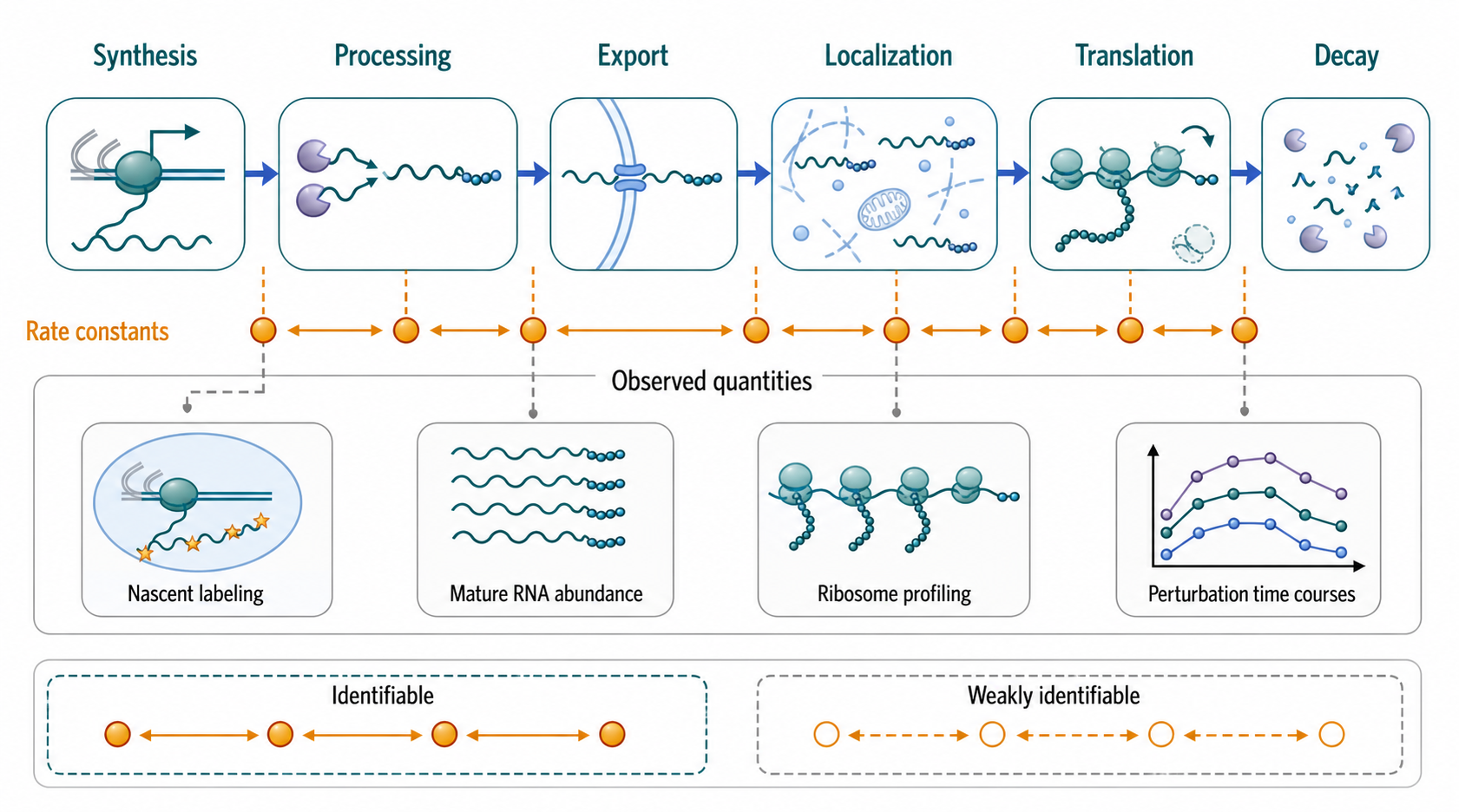
Figure 146.2. Kinetic Model of mRNA Life History. A transcript can be modeled as a molecule moving through production, processing, export, localization, translation, and decay states. Nascent labeling constrains synthesis and processing rates, mature RNA-seq constrains abundance, fractionation and imaging constrain localization, ribosome profiling constrains translation, and time-course perturbations constrain degradation. Some parameters remain weakly identifiable unless the experiment measures time, compartment, or perturbation response directly.
Ordinary differential equation models describe how average concentrations change over time. They are useful when molecule numbers are high enough that stochastic fluctuations can be approximated by continuous variables. A model might include nuclear pre-mRNA, nuclear mature mRNA, cytoplasmic mRNA, translating mRNA, and degraded products. Rate constants can represent splicing, export, translation initiation, and decay. The output can be predicted time courses after stimulation or perturbation. The limitation is that average models hide cell-to-cell variability and bursty transcription.
Stochastic models represent probability distributions over molecule numbers and states. Transcription often occurs in bursts because promoters switch between active and inactive states. In single cells, two cells with the same average transcription rate can have different burst frequency, burst size, and noise. Stochastic birth-death models, chemical master equations, and simulations can therefore explain why an RNA appears in a subset of cells or why a regulatory circuit produces heterogeneous responses. The limitation is that stochastic models often require more data and stronger assumptions than deterministic models.
State-space models represent hidden biological states that generate observed data. A hidden state might be the true abundance of a transcript over time, while observations are noisy RNA-seq counts. In a single-cell trajectory, a hidden variable might represent progression through differentiation or activation. State-space models can combine time courses, lineage information, and perturbations, but hidden states can become biological fictions if they are not anchored by independent measurements. A pseudotime coordinate is not a clock unless validated with real time, lineage tracing, or known sequence of events.
Bayesian hierarchical models are useful when data come from many genes, cells, donors, tissues, or species. They can share information across related units while estimating uncertainty for each unit. For example, decay rates might be modeled as gene-specific values drawn from a distribution influenced by UTR length, codon optimality, miRNA sites, RNA-binding protein motifs, and cell state. Such models can prevent overfitting for poorly measured genes, but they also encode priors. A prior that assumes most genes behave similarly may obscure rare but important regulatory programs.
Machine-learning models can predict RNA abundance, splicing, translation, localization, or decay from sequence, structure, chromatin, cell state, or perturbation features. Their strength is flexible pattern recognition. Their weakness is that a predictor can work for the wrong reason. A model that predicts high translation from a coding sequence may rely on gene family, expression level, or annotation artifacts rather than causal codon features. A model that predicts RNA localization may learn cell-type markers instead of transport elements. Quantitative RNA biology therefore asks not only whether a model predicts, but what intervention would test the learned relationship.
Table 146.2. Model Classes for RNA Life-Cycle Dynamics. Deterministic, stochastic, hierarchical, state-space, agent-based, and machine-learning models represent different RNA-life-cycle questions and assumptions; predictive fit does not by itself validate mechanism.
| Model class | RNA-system use | Evidence or caveat |
|---|---|---|
| Ordinary differential equation models | Describe average changes in RNA states such as nuclear pre-mRNA, mature RNA, exported RNA, translating RNA, and degraded products. | Useful for time courses and rate hypotheses, but average trajectories hide bursty transcription and cell-to-cell heterogeneity. |
| Stochastic birth-death and chemical-kinetic models | Represent probability distributions over promoter states, molecule counts, burst frequency, burst size, processing, and decay. | Better for single-cell variation and noisy regulatory circuits, but often require richer data and stronger assumptions. |
| State-space and trajectory models | Infer hidden biological states from noisy observations, such as latent RNA abundance over time or progression through activation or differentiation. | Hidden coordinates can become biological fictions unless anchored by time courses, lineage tracing, markers, perturbations, or independent measurements. |
| Bayesian hierarchical models | Share information across genes, cells, donors, tissues, species, or perturbations while estimating uncertainty for each unit. | Priors can stabilize weakly measured parameters but can also smooth away rare regulatory programs or context-specific effects. |
| RNA processing and isoform models | Predict splice choices, isoform abundance, transcript-end use, nonsense-mediated decay sensitivity, or long-read-supported transcript structures. | Short reads can quantify known junctions but may not resolve full molecules; long reads resolve structure but can have depth and error limitations. |
| Translation and decay kinetic models | Separate initiation, elongation, pausing, termination, protein stability, deadenylation, decapping, cleavage, and exonucleolytic decay. | Summary measures such as half-life or footprint density can hide multi-step kinetics and pathway switching. |
| Machine-learning predictors | Predict abundance, splicing, translation, localization, decay, or perturbation response from sequence, structure, chromatin, cell state, and context features. | Prediction can succeed for noncausal reasons such as gene family, batch, annotation artifacts, expression level, or cell-type markers. |
| Agent-based or rule-based simulations | Explore how local RNA rules, compartmentalization, cell-state mixtures, or interacting regulators generate population-level behavior. | Simulation output depends on chosen rules and parameters; agreement with a pattern is weaker than identifiable rates or perturbation-tested mechanism. |
Identifiability is the bridge between modeling and experimental design. Suppose mature mRNA abundance doubles after a stimulus. A model with synthesis and decay parameters can fit the observation in multiple ways. Nascent RNA labeling can constrain synthesis. A transcriptional shutoff or metabolic pulse-chase can constrain decay. Nuclear and cytoplasmic fractionation can constrain export. Ribosome profiling can constrain translation. Imaging can constrain localization and cell-to-cell variation. A perturbation of a suspected RNA-binding protein can test whether a sequence element is relevant. Each additional measurement narrows the model, but no measurement is assumption-free.
Consider a concrete example: an inflammatory cytokine mRNA in macrophages. After stimulation, chromatin accessibility increases near the locus, nascent RNA rises within minutes, mature RNA peaks later, ribosome occupancy follows, and protein secretion appears after translation and trafficking. A negative regulator may later accelerate mRNA decay. A model that includes only mature RNA abundance would see a pulse. A kinetic model can separate early synthesis, delayed processing, translation, and late decay. A perturbation that removes an AU-rich element in the 3′ UTR can test whether rapid decay shapes the pulse. A rescue experiment that restores the element can strengthen causal interpretation.
RNA processing models add combinatorial complexity. Alternative splicing is not just inclusion or skipping of an exon; it can involve splice-site strength, RNA polymerase elongation, RNA secondary structure, RNA-binding protein occupancy, chromatin state, cell type, and surveillance of isoforms. A splicing model may predict percent-spliced-in values, isoform abundances, protein domains, or nonsense-mediated decay sensitivity. Long-read sequencing helps connect splice choices across a molecule, but long-read depth, error profiles, and library preparation biases must be considered. Short-read splice-junction counts can be precise for known junctions but ambiguous for full-length isoforms.
Translation models must distinguish initiation, elongation, termination, ribosome recycling, and protein stability. Codon usage and tRNA pools can influence elongation and cotranslational folding. Upstream open reading frames can reduce or conditionally enhance downstream translation. RNA structure near the 5′ end can affect scanning or initiation. miRNAs and RNA-binding proteins can repress translation, promote decay, or do both. Ribosome profiling can report footprints, but footprint density is a composite signal. A stalled ribosome can increase local footprint density while decreasing productive protein output.
Decay models connect sequence features to enzyme pathways. Deadenylation, decapping, exonucleolytic decay, endonucleolytic cleavage, nonsense-mediated decay, no-go decay, nonstop decay, codon optimality-mediated decay, miRNA-associated decay, and specialized nuclear surveillance each impose different dependencies. A decay model should specify whether it describes bulk half-life, pathway entry, enzyme recruitment, deadenylation rate, decapping rate, or final exonucleolytic degradation. Half-life is a useful summary, but it can hide multi-step kinetics.
The evidence boundary is that models are not mechanisms by themselves. A model can show that a proposed mechanism is consistent with data, or that two mechanisms are distinguishable under a planned experiment. A model cannot prove that an unmeasured molecule acted. Strong quantitative systems RNA biology uses models to design decisive measurements rather than to decorate descriptive data.
146.3. Network Motifs, Feedback, Robustness, Oscillation, and Cell-State Transitions
RNA regulation is organized into networks because each RNA molecule can be both a target and a regulator. An mRNA encodes a protein that may regulate transcription, splicing, translation, or decay of other RNAs. A miRNA targets many mRNAs, and those targets can include transcription factors, signaling proteins, RNA-binding proteins, and feedback regulators. A bacterial small RNA can repress one mRNA while indirectly activating another by titrating an RNA-binding protein or changing metabolic state. A splicing factor can regulate its own transcript to produce a nonproductive isoform. These connections create motifs that recur across systems.
Negative feedback occurs when a regulatory output reduces its own production or activity. In RNA biology, a classic form is autoregulation by an RNA-binding protein that binds its own pre-mRNA or mRNA. If the protein becomes abundant, it can alter splicing, translation, localization, or decay of its own transcript, thereby reducing further protein accumulation. Negative feedback can buffer noise and stabilize abundance. However, delayed negative feedback can create pulses or oscillations if the feedback is strong and slow relative to production and decay. The same wiring can therefore produce stability or rhythmic behavior depending on kinetic parameters.
Positive feedback occurs when an output promotes its own production or stabilizes its own state. A transcription factor induced by a translated mRNA may activate more of the same mRNA. A cell-state regulator may repress a miRNA that would otherwise repress that regulator. Positive feedback can create memory and bistability, where cells occupy one of two stable states. The boundary case is amplification without true memory. If the feedback disappears quickly when the stimulus is removed, the system may be only transiently amplified rather than bistable.
Feed-forward loops involve an upstream regulator that controls a target through two paths. In a coherent feed-forward loop, both paths have the same sign; in an incoherent feed-forward loop, one path activates and the other represses. RNA regulators often participate in incoherent motifs. For example, a transcription factor may activate an mRNA and also activate a miRNA or RNA-binding protein that represses the same mRNA later. This architecture can create pulses, adaptation, or noise filtering. A bacterial small RNA can similarly create threshold behavior when target mRNAs compete for a limited regulatory RNA or chaperone.
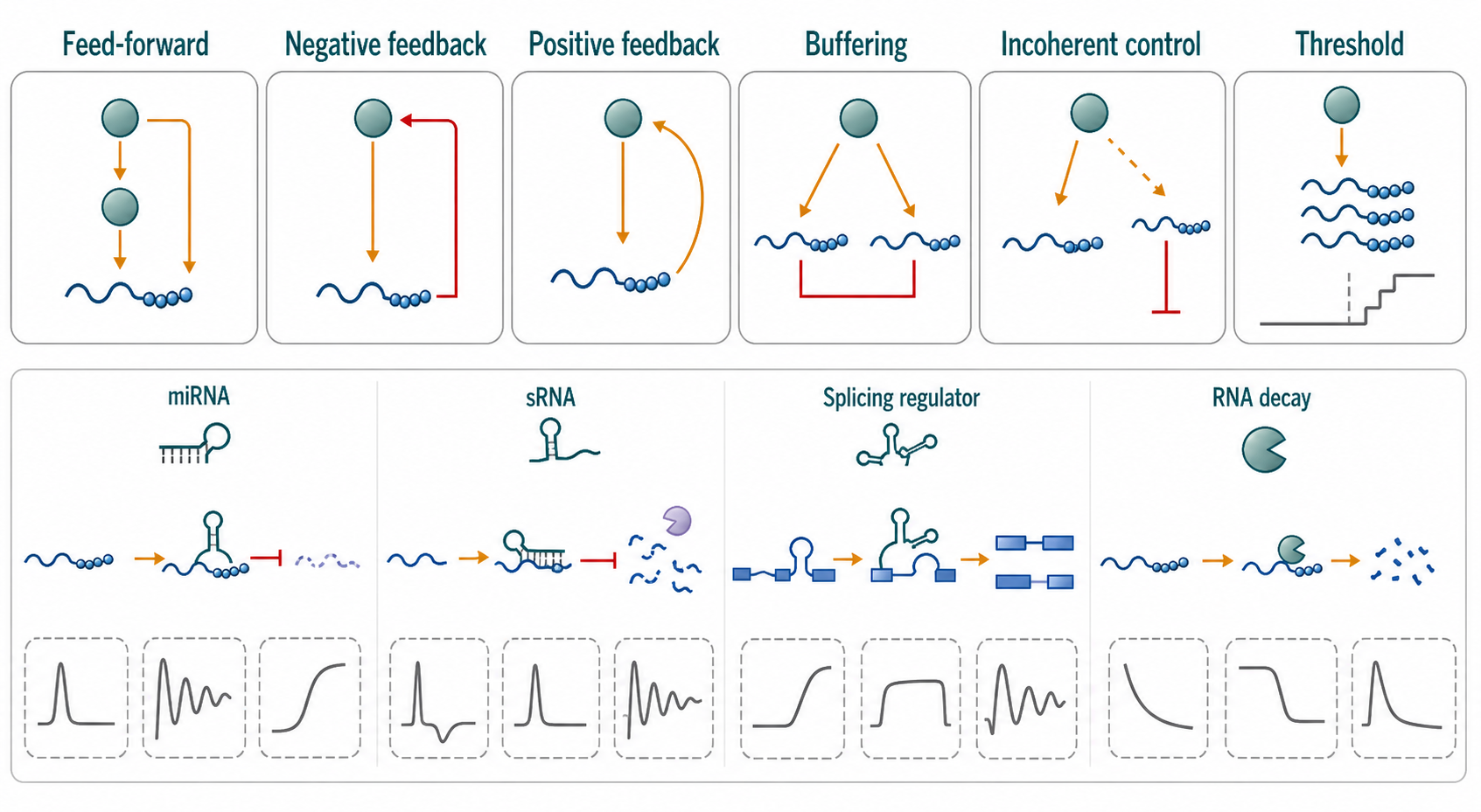
Figure 146.3. RNA-Centered Network Motifs and Dynamic Behaviors. RNA regulation participates in common network motifs. miRNA-mediated repression can buffer noisy transcription, bacterial small RNAs can create threshold-like responses, splicing regulators can generate feedback on their own isoforms, and RNA decay can tune pulse duration. The same motif can stabilize a state, sharpen a transition, or create oscillatory behavior depending on rate constants, delays, and molecular saturation.
Robustness means that a system preserves a function despite perturbations. In RNA biology, robustness can arise from redundant RNA-binding proteins, multiple miRNA sites, buffering by RNA decay, compensatory transcription, alternative isoforms, and distributed control across many weak interactions. Robustness is not always desirable from a therapeutic or engineering perspective. A disease-relevant RNA program may resist intervention because several mechanisms compensate. Conversely, a synthetic RNA circuit may fail because the host cell buffers or silences the introduced component.
Oscillation requires more than periodic expression. A true oscillator has a mechanism that regenerates cycles, such as delayed negative feedback, coupled feedback loops, or rhythmic external forcing. RNA contributes to oscillatory systems by controlling delays and degradation rates. Short mRNA half-lives can allow rapid cycles; long half-lives can smooth fluctuations. Alternative splicing, nuclear retention, translational delay, and protein turnover can add phase shifts. Evidence for RNA involvement in oscillation should distinguish RNA rhythms that drive the cycle from RNA rhythms that are downstream markers of another clock.
Cell-state transitions are coordinated changes in molecular and functional identity. Differentiation, immune activation, stress response, epithelial-mesenchymal transition, infection response, and tumor progression all include RNA changes. Single-cell RNA-seq often represents transitions as trajectories or clusters. These representations are useful, but a cluster is not automatically a state and a trajectory is not automatically a lineage. A cell-state claim becomes stronger when transcriptomic structure is supported by time courses, lineage tracing, spatial organization, protein markers, chromatin changes, perturbation response, or functional assays.
RNA mechanisms can drive state transitions by changing thresholds. A miRNA can repress low-level leaky expression of a fate regulator while allowing high-level induced expression to pass a threshold. An RNA-binding protein can switch splicing from one isoform program to another. A change in mRNA decay can shorten or extend a pulse of signaling. A localized mRNA can restrict protein synthesis to a cellular compartment, enabling local synaptic, developmental, or polarity decisions. A stress granule can temporarily store or triage RNAs, although association with a granule should not be overinterpreted as proof of repression or protection without direct measurement.
Network inference from RNA data faces a central problem: correlation is dense. Genes in the same pathway, cell type, cell-cycle phase, or batch can be coexpressed even when none directly regulates the others. A transcription factor mRNA can correlate with its targets, but the active molecule is the protein, often modified and localized. A miRNA can anticorrelate with a target, but many real targets show weak or context-specific abundance changes. RNA-binding protein motifs can be enriched in a gene set, but motif enrichment does not prove binding or regulation. Strong network models combine prior knowledge, perturbations, temporal ordering, and direct binding or biochemical evidence.
The evidence basis for network dynamics often requires perturbing nodes and measuring response. If removing an RNA-binding protein changes splicing of its own transcript and changes protein abundance in a direction consistent with feedback, the feedback model is plausible. If restoring an RNA-binding site rescues regulation, the model becomes stronger. If a time-course shows delayed repression after activation, an incoherent feed-forward model gains support. If single-cell measurements show reduced variance after introducing a miRNA site, a buffering model is supported. Each claim should specify the system, time scale, and output.
The cross-chapter handoff is to regulation grammar and experimental design. Chapters on mRNA architecture, miRNAs, bacterial small RNAs, ribosome profiling, and perturbation screens provide molecular details. This chapter emphasizes that network behavior depends on combining those details with quantitative dynamics.
146.4. Evolutionary Systems Biology and Comparative Transcriptomics
Evolutionary systems biology asks how regulatory systems change while organisms remain viable and adapted. Comparative transcriptomics measures RNA programs across species, strains, populations, tissues, developmental stages, or environmental conditions. The simplest comparison asks whether orthologous genes have similar expression. More advanced comparisons ask whether isoforms, UTRs, RNA structures, RNA-binding protein motifs, miRNA target sites, cell-type programs, perturbation responses, and network modules are conserved or rewired.
Orthology is the first prerequisite. Orthologous genes descend from a common ancestral gene through speciation, while paralogous genes arise by duplication. Expression comparison across paralogs can be biologically meaningful, but it answers a different question than ortholog comparison. RNA genes and noncoding RNAs add complexity because sequence conservation can be low, structure can be conserved without obvious primary-sequence similarity, and lineage-specific RNAs can be abundant. Annotation differences can create false evolutionary claims. A transcript absent from one species may be truly absent, unannotated, expressed in an unsampled condition, or too divergent for detection.
Cell-type alignment is the second prerequisite. A liver sample from one species and a liver sample from another may contain different proportions of hepatocytes, immune cells, endothelial cells, stromal cells, and developmental states. Single-cell atlases can help align cell types, but cross-species cell-type names can be misleading. A cell type may have conserved function but altered markers. Another cell type may be split into subtypes in one lineage and not another. Comparative systems RNA biology should therefore align morphology, function, marker genes, developmental origin, and regulatory programs when possible.
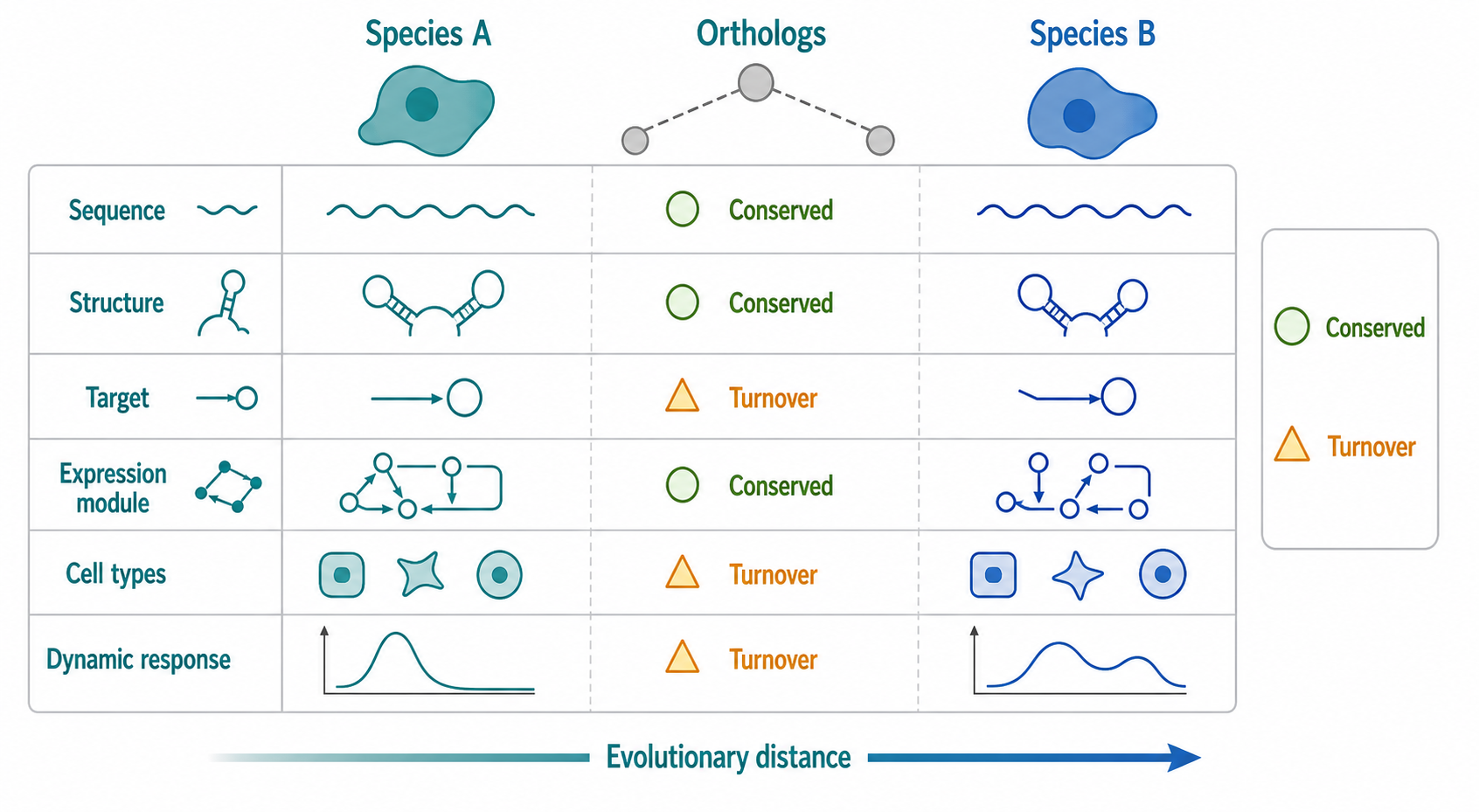
Figure 146.4. Comparative Systems RNA Biology Across Evolutionary Distances. Comparative RNA systems analysis can align orthologous genes, conserved RNA structures, regulatory motifs, cell types, perturbation responses, and network modules. Conservation at one layer does not guarantee conservation at another layer: a transcript may keep protein-coding function while changing untranslated-region regulation, or a regulatory output may remain conserved while the responsible RNA motif turns over.
Regulatory conservation occurs at several layers. A coding gene may have conserved expression but different UTR motifs. A miRNA family may be conserved, but individual target sites can turn over. A splicing event may be conserved in a tissue even when the intronic regulatory sequence changes. A stress response may induce homologous pathways with different timing or amplitude. A riboswitch may conserve ligand response while sequence changes preserve structure. A bacterial small-RNA network may preserve a physiological output through different small RNAs in different lineages. The level of conservation should be stated explicitly.
Comparative transcriptomics can reveal evolutionary novelty. New promoters, transposable element insertions, alternative polyadenylation sites, splice sites, circular RNAs, antisense transcripts, and noncoding RNAs can create lineage-specific regulation. Some innovations become functional; others are transcriptional noise or weakly selected byproducts. Evidence for function should follow the same standards used within one organism: reproducible expression, regulated processing, conservation when expected, perturbation phenotype, mechanism, and exclusion of annotation artifacts.
Evolutionary turnover creates an important misconception. Lack of sequence conservation does not prove lack of function, especially for regulatory RNAs whose structure, expression, or target logic may be conserved in ways that are difficult to align. At the same time, expression does not prove function. A systems view keeps both cautions. It asks whether the RNA participates in a conserved or lineage-specific system, whether perturbation changes an organismal or cellular phenotype, and whether the molecular mechanism is plausible.
Comparative models must handle phylogeny. Species are not independent samples if they share ancestry. A trait shared by two closely related species may reflect inheritance rather than repeated adaptation. A trait present in distant species may reflect deep conservation, convergence, or incomplete sampling. Phylogenetic comparative methods can help separate these explanations, but they require careful species trees, trait definitions, and uncertainty estimates. RNA regulation adds additional uncertainty because transcript annotations and expression data are uneven across species.
A concrete example is the comparison of immune-response RNA programs across mammals. Some inflammatory genes show conserved induction, but enhancer usage, UTR length, miRNA targeting, alternative splicing, and decay kinetics can differ. A bulk comparison may conclude that a response is not conserved because the timing differs. A time-course model may reveal that the same pathway is activated with shifted kinetics. A single-cell comparison may reveal that species differ in cell composition rather than cell-intrinsic response. A perturbation may show that the same transcription factor is required even when downstream RNA features have changed.
Evolutionary systems biology also includes population variation within species. Genetic variants can alter splicing, RNA abundance, allele-specific expression, RNA modification, translation, and RNA decay. Expression quantitative trait loci, splicing quantitative trait loci, allele-specific ribosome profiling, and proteogenomic integration can link genotype to RNA system behavior. Causal interpretation requires care because linked variants, cell composition, environment, and technical batch can confound associations. Functional validation of candidate variants often requires reporter assays, genome editing, or allele-specific perturbation.
The handoff to AI and causal inference is direct. Comparative data create large, structured matrices with missing values, annotation uncertainty, and evolutionary dependence. AI models can help align sequences, predict regulatory elements, infer cell correspondences, and propose conserved modules. Causal inference is needed to distinguish historical association from regulatory mechanism.
146.5. AI, Causal Inference, Perturbation Modeling, Organism-Scale RNA Knowledge Graphs, and Validation Loops
Artificial intelligence is useful in systems RNA biology because the data are high-dimensional, multimodal, sparse, and structured. Sequence models can learn patterns in RNA sequence, UTRs, splice sites, coding regions, modification contexts, and RNA-binding protein motifs. Graph models can represent interactions among genes, RNAs, proteins, cell types, diseases, and perturbations. Generative models can impute missing modalities, predict perturbation responses, design sequences, or propose regulatory hypotheses. Foundation-style models can produce embeddings that summarize sequence or expression context. These tools are powerful, but their outputs are predictions, not mechanisms.
Causal inference asks a different question from prediction. Prediction estimates an outcome from observed variables. Causal inference estimates the effect of an intervention. If a model predicts that an RNA-binding protein and a target mRNA are associated with a cell state, that is not yet a causal claim. A causal claim would ask what happens to the cell state if the RNA-binding protein is removed, if its binding site is mutated, if the target RNA is rescued, or if the pathway is perturbed at a defined time. Causal inference depends on assumptions about confounders, mediators, colliders, time ordering, measurement error, and intervention specificity.
Box 146.3. Prediction Is Not the Intervention
Prediction Is Not the Intervention
An AI model can discover a pattern that is useful and still not discover the causal mechanism. For example, a sequence model may predict that a 3′ UTR belongs to unstable mRNAs because the UTR carries AU-rich motifs, because the gene family is usually short-lived, or because the training labels came from one cell type. These explanations imply different experiments. To move from prediction to mechanism, specify the proposed intervention: mutate the motif, change the RNA-binding protein, alter the endogenous locus, rescue the RNA element, or test the response in a new context. Then specify the readout that matches the claim: decay kinetics for stability, splice isoforms for splicing, ribosome engagement plus protein output for translation, or chromatin state plus transcription for chromatin-linked regulation. Feature importance is a prompt for experiments, not a substitute for them.
Directed acyclic graphs are one way to state causal assumptions. A graph might say that stimulation changes transcription-factor activity, transcription-factor activity changes nascent RNA synthesis, RNA-binding protein abundance changes mRNA decay, and both pathways affect mature RNA abundance. The graph might also include cell-cycle state as a confounder because cell cycle affects both RNA abundance and protein abundance. The value of such a graph is not that it captures every molecule. The value is that it makes assumptions explicit enough to test or criticize.
Perturbation modeling uses experimental interventions to learn response. In CRISPR screens, the perturbation may remove a gene. In CRISPR interference, it may reduce transcription. In RNA interference, it may deplete an RNA with possible off-target effects. In antisense experiments, it may block splicing, induce RNase H cleavage, or alter translation. In drug perturbations, it may inhibit a protein or pathway with dose-dependent and off-target actions. In environmental perturbations, it may change many upstream variables at once. The model must know what intervention was attempted, how strong it was, when it was measured, and which cells survived.
Perturb-seq-like assays are especially important because they connect genetic perturbation to single-cell transcriptomic outcomes. They can map regulators to target programs, identify cell-state shifts, and train models that predict responses to unseen perturbations. However, these assays often measure RNA outcomes but not protein activity, chromatin state, metabolite state, or long-term phenotype. Guide efficiency varies. Strong perturbations can select for surviving cells. Double perturbations are much harder to predict than single perturbations. A perturbation model trained in one cell line may fail in primary tissue, another species, or a different environmental context.
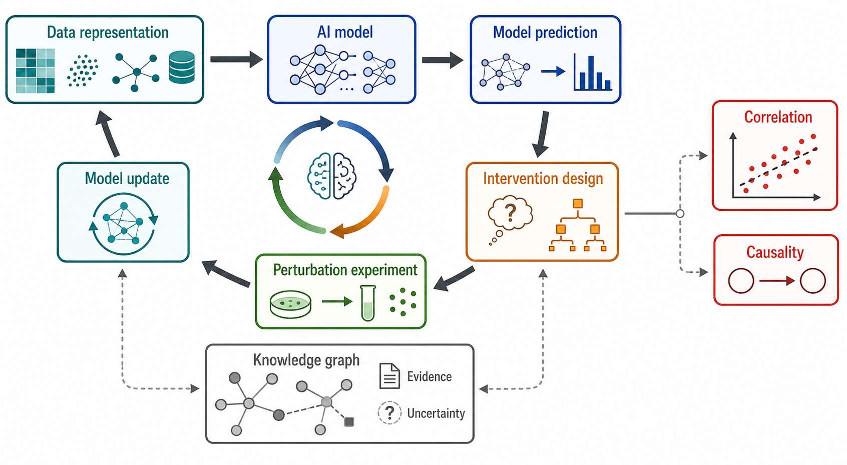
Figure 146.5. AI-Assisted Causal Inference and Validation Loop. AI-assisted RNA systems biology is most reliable when predictive models are embedded in a causal validation loop. Observational multi-omics data suggest hypotheses; perturbation data test interventions; causal models distinguish correlation from response; and curated knowledge graphs preserve entities, assumptions, evidence, and unresolved contradictions for the next experiment.
AI-assisted causal inference is most reliable as a loop. Observational data suggest candidate regulators, motifs, latent states, or pathways. A model ranks hypotheses and proposes interventions. A perturbation experiment tests a subset. The results update the model. A knowledge graph records the entity, intervention, context, effect, evidence type, and uncertainty. The next experiment is designed to distinguish remaining alternatives. This loop is slower than making predictions on an atlas, but it is how integrated data become mechanistic knowledge.
Organism-scale RNA knowledge graphs can support this loop when their semantics are precise. Nodes can represent genes, transcript isoforms, RNA elements, RNA modifications, proteins, complexes, pathways, cell types, tissues, diseases, phenotypes, perturbations, methods, datasets, and publications. Edges can represent physical binding, enzymatic modification, transcriptional regulation, splicing regulation, translation regulation, decay regulation, localization, coexpression, genetic interaction, disease association, orthology, or evidence support. A graph that labels every edge as “related to” is not adequate for causal reasoning.
Knowledge graphs also need provenance. A CLIP-seq peak near an RNA-binding protein motif is not the same as biochemical binding to a purified RNA fragment. A reporter assay is not the same as regulation at the endogenous locus. A genome-wide association is not the same as a validated disease mechanism. A curated edge should record the organism, cell type, condition, molecule form, assay, perturbation, effect size when available, citation, and uncertainty. Deprecated names and transcript annotation versions matter because RNA entities change across databases.
Table 146.3. Evidence Standards for Causal Claims in Systems RNA Biology. Causal evidence strengthens from association through temporal precedence, perturbation, rescue, epistasis, cross-context replication, and biochemical mechanism; each rung supports a different claim ceiling.
| Evidence rung | What it supports | Caveat for causal claims |
|---|---|---|
| Coexpression, anticorrelation, or motif enrichment | Suggests candidate regulators, targets, cis-elements, pathways, or cell-state associations. | Lowest causal strength because shared regulators, composition, batch, annotation, or indirect effects can create the same pattern. |
| Temporal precedence | Shows that a regulator, RNA state, or molecular layer changes before a proposed target or phenotype. | Supports ordering but not sufficiency; both variables may still respond to an unmeasured upstream cause. |
| Direct binding or occupancy | Provides physical plausibility through CLIP-like maps, chromatin occupancy, motif-dependent binding, or biochemical interaction evidence. | Binding does not prove regulation, and genome-wide occupancy differs from purified-component mechanism. |
| Perturbation response | Tests whether CRISPR, RNAi, antisense, drug, environmental, or sequence perturbation changes the predicted RNA outcome. | Intervention strength, timing, off-target effects, viability, and cell-state composition determine interpretability. |
| Rescue or allele restoration | Tests specificity by restoring the RNA, regulator, motif, isoform, or domain expected to repair the phenotype. | Rescue must match expression, timing, localization, and molecular form closely enough to avoid artificial compensation. |
| Epistasis and ordered perturbations | Places regulators, RNA elements, pathways, or processing steps in a causal order. | Requires well-controlled single and combined interventions; broad toxicity or saturation can obscure order. |
| Biochemical or mechanistic reconstitution | Tests whether purified components or minimal systems can execute binding, modification, processing, translation control, or decay. | High mechanistic specificity, but in vitro conditions may omit cellular cofactors, compartment effects, or competing pathways. |
| Cross-context replication | Asks whether the mechanism holds across donors, cell types, tissues, species, perturbation types, or time points. | Generality is stronger when contexts are biologically independent and not linked by shared batch, database rule, or annotation source. |
| Organismal, disease, or clinical phenotype | Connects the RNA mechanism to tissue function, development, pathogenesis, therapy, or patient-relevant outcome. | Phenotypic relevance does not by itself identify the molecular step; mechanism still needs RNA-specific evidence. |
| Knowledge-graph provenance | Records entity, context, assay, perturbation, effect, uncertainty, and citation for each edge. | A graph edge labeled only as related to is inadequate for causal reasoning even when the underlying association is real. |
Causal evidence can be arranged as a ladder. At the lower end, coexpression or motif enrichment suggests a hypothesis. Temporal precedence adds information: a regulator changes before a target. Direct binding or occupancy supports physical plausibility. Perturbation shows response. Rescue tests specificity. Epistasis places components in order. Biochemical reconstitution shows that purified components can execute a mechanism. Cross-context replication tests generality. Clinical or organismal evidence connects the mechanism to phenotype. Not every RNA claim needs every rung, but strong causal claims should not rest only on the lowest rungs.
AI methods can fail in RNA-specific ways. Sequence models may learn taxonomic or gene-family signals rather than causal elements. Expression models may learn batch, cell-cycle, or dissociation stress. Perturbation models may learn average viability responses rather than specific regulatory mechanisms. Knowledge-graph models may infer plausible edges because well-studied genes are densely annotated. Imputation methods may hallucinate smooth expression where rare cell states or transient RNA species exist. A high benchmark score is not enough if the benchmark rewards shortcuts.
Validation should be designed around the claim. If the claim is that a UTR element controls mRNA decay, validation should mutate the element in its native context or a suitable reporter, measure decay kinetics, and test dependence on the proposed regulator. If the claim is that a noncoding RNA organizes a chromatin state, validation should perturb the RNA, rescue the RNA or relevant domain, measure chromatin and expression effects, and rule out transcriptional interference if necessary. If the claim is that an AI model can predict perturbation response, validation should include held-out perturbations, held-out contexts, and prospective experiments.
The boundary between AI assistance and scientific inference should remain explicit. AI can help choose candidates, summarize evidence, identify contradictions, design perturbations, and update graphs. It cannot remove the need for well-designed experiments, because biological causality is about interventions in physical systems.
146.6. Data Integration Limits, Batch Effects, Missing Modalities, Benchmark Design, and Experimental Validation
Systems RNA biology is vulnerable to artifacts because integration multiplies assumptions. A single RNA-seq dataset has library preparation bias, mapping ambiguity, normalization choices, gene annotation dependence, and sampling variance. Adding proteomics introduces protein extraction, digestion, peptide detectability, missing values, and dynamic-range issues. Adding metabolomics introduces chemical coverage, ion suppression, annotation uncertainty, and batch effects. Adding spatial data introduces tissue processing, segmentation, capture efficiency, and resolution limits. Adding perturbations introduces intervention variability. Integration can clarify biology, but it can also align errors.
Batch effects are systematic technical differences unrelated to the intended biology. A batch can be a sequencing run, library kit, mass spectrometry day, tissue processing protocol, dissociation method, operator, center, reagent lot, or computational pipeline. Batch correction methods can reduce unwanted variation, but they can also remove real biology if the biological variable is confounded with batch. If all diseased samples were processed in one batch and all controls in another, no statistical method can fully distinguish disease from processing without additional assumptions or data.
Missing modalities are often informative rather than random. Proteomics may be missing for rare cell populations because too little material was available. Spatial data may be missing for fragile tissues. Metabolomics may be absent for single-cell perturbation screens because the assay is destructive or not sensitive enough. Long-read isoform data may exist only for selected tissues. A model that treats missingness as random can overstate confidence. A good integration report states which layers were measured in the same sample, matched samples, similar samples, or public reference samples, and which layers were imputed.
Compositional effects are another recurrent failure. A bulk tumor sample can show increased expression of an immune RNA program because more immune cells entered the tumor, because tumor cells activated immune-like pathways, or because both occurred. A treated tissue can show decreased neuronal mRNAs because neurons died, because neurons changed expression, or because non-neuronal cells expanded. Single-cell data can help, but dissociation bias can change apparent composition. Spatial data can help, but spatial resolution and segmentation can blur cell boundaries. The safest interpretation connects molecular change to cell identity and abundance.
Annotation drift affects RNA systems more than many protein-centered analyses. Transcript models change as new splice isoforms, 3′ ends, noncoding RNAs, pseudogenes, and repeats are annotated. A read assigned to one transcript in one annotation version may be assigned differently in another. Cross-species annotations are uneven. Noncoding RNA names and boundaries are especially unstable. Systems studies should record genome build, annotation version, transcript identifiers, quantification method, and filtering rules. Knowledge graphs should preserve these identifiers rather than only gene symbols.
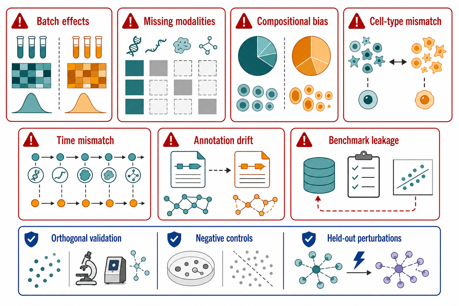
Figure 146.6. Failure Modes in Multi-Omics Integration. Integrated RNA systems models can fail for reasons that are not biological. Technical batches, incomplete modality coverage, destructive assays performed on different cells, sparse measurements, cell-type composition shifts, reference-annotation changes, and circular benchmark design can create apparent mechanisms. Validation requires orthogonal assays, held-out perturbations, prospective predictions, and explicit negative controls.
Benchmark design is a scientific problem, not an administrative afterthought. A benchmark for RNA integration should test the intended use case. If a method claims to integrate RNA and protein across tissues, the test set should include held-out tissues or donors. If a model claims to predict effects of unseen perturbations, the test set should hold out perturbations, not only random cells from perturbations already seen during training. If a model claims sequence-based generalization, homologous sequences, duplicated genes, or near-identical reporter constructs should not leak between training and test sets. If a knowledge-graph model predicts missing edges, edges derived from the same publication or database rule should be split carefully.
Benchmark leakage can be subtle. A model may appear to predict RNA-binding protein targets because the test labels were derived from motif scans that the model also uses as features. A perturbation model may appear to generalize because cells from the same perturbation appear in both training and test sets. A sequence model may appear to discover regulatory grammar because paralogous genes share both sequence and labels across splits. An imputation model may appear accurate because the evaluation masks observed values at random rather than holding out an entire modality, tissue, or condition. Strong benchmarks use negative controls and biologically meaningful held-out structure.
Table 146.4. Benchmark and Validation Design Rules. Reliable evaluation of RNA integration and perturbation models requires leakage-resistant splits, external contexts, calibrated metrics, ablations, uncertainty, and reproducible data lineage; one benchmark score is not general validity.
| Design rule | What it protects | Failure prevented |
|---|---|---|
| Align modalities by biological question | Decide whether the analysis aligns samples, cells, neighborhoods, genes, pathways, perturbations, time points, or latent states. | A matrix merge can look integrated while combining measurements that observe different molecules, scales, or time windows. |
| Record same-sample versus matched-sample evidence | Distinguish layers measured in the same sample, matched samples, similar reference samples, or imputed reference data. | Missing modalities are often nonrandom because assay compatibility, tissue availability, cost, and sensitivity determine what is measured. |
| Block or balance batch structure | Spread conditions, donors, tissues, perturbations, and sequencing or mass-spectrometry runs across batches when possible. | Batch correction can remove true biology when batch and biology are confounded. |
| Model cell composition explicitly | Separate changes in cell abundance from cell-intrinsic RNA regulation using single-cell, spatial, marker, or deconvolution evidence. | Bulk shifts can reflect immune infiltration, cell death, expansion, or dissociation bias rather than RNA regulation in the same cell type. |
| Preserve genome and transcript annotation versions | Record genome build, transcript identifiers, quantification method, filtering rules, and deprecated names. | Annotation drift is especially important for isoforms, 3′ ends, noncoding RNAs, repeats, and cross-species comparisons. |
| Hold out the right biological unit | Match the test split to the claim, such as held-out donors, tissues, species, perturbations, cell types, time points, or modalities. | Random cell-level splits can overstate performance when the same perturbation, donor, or context appears in training and test data. |
| Prevent sequence and annotation leakage | Keep paralogous genes, homologous sequences, near-identical reporter constructs, target-derived features, and shared database rules from crossing train-test boundaries. | Leakage can make a model appear to learn regulatory grammar or binding specificity when it is exploiting reused labels or similarity. |
| Use negative controls and null tasks | Include scrambled labels, irrelevant features, inactive guides, neutral sequence variants, and batch-aware reanalyses. | Negative controls reveal shortcuts, overfitting, viability-driven responses, and integration methods that align errors. |
| Validate prospectively when claiming prediction | Test model-selected regulators, RNA elements, perturbations, or contexts in experiments not used for training or benchmark construction. | Prospective success is stronger than retrospective fit, especially for AI perturbation models and organism-scale knowledge graphs. |
| Use orthogonal readouts for mechanism | Pair predictions with independent assays such as RT-PCR, long-read sequencing, reporter mutation, imaging, biochemical binding, proteomics, or rescue. | Orthogonal validation should match the claim: splicing, localization, translation, decay, chromatin effect, or causal perturbation response. |
| Preserve negative and contradictory evidence | Track failed rescues, absent binding, null motif mutations, reanalysis failures, and context-specific nonreplication. | Negative evidence prevents attractive integrated narratives from hardening into unsupported mechanism. |
Experimental validation should be proportional to claim strength. A descriptive atlas can be validated by technical replication, marker agreement, spatial consistency, and comparison with known biology. A predictive model can be validated by held-out data and prospective prediction. A causal mechanism requires intervention. A therapeutic or disease claim requires relevant biological models, dose response, safety and specificity assessment, and ideally clinical or patient-derived evidence when appropriate. An evolutionary claim requires phylogenetic and comparative controls. A knowledge-graph claim requires evidence provenance and manual review for high-impact edges.
Orthogonal validation means using a different measurement principle. If RNA-seq suggests altered splicing, reverse-transcription PCR, long-read sequencing, or targeted isoform assays can validate the event. If ribosome profiling suggests translation of an upstream open reading frame, reporter mutation, proteomics, or epitope tagging can test protein production or regulatory effect. If a CLIP experiment suggests binding, electrophoretic mobility shift, in vitro binding, mutational reporter assays, or endogenous editing can test binding and function. If spatial transcriptomics suggests localized RNA, single-molecule fluorescence in situ hybridization can validate localization.
Negative evidence is valuable. Failure to rescue a phenotype, absence of binding in a biochemical assay, lack of effect after endogenous motif mutation, or disappearance of a signal after batch-aware reanalysis can prevent a weak story from hardening into false mechanism. Systems RNA biology should preserve negative and contradictory evidence because integrated models otherwise become biased toward attractive narratives.
The final boundary is biological scale. An organism-scale model is not a complete organism. It is a structured approximation built from measured variables, assumptions, and missing layers. A useful model tells researchers where it is confident, where it is extrapolating, which variables are unobserved, which claims are causal, and which experiments would change the conclusion.
Recent Consensus
The current consensus, stated without pretending complete local citation support, is that RNA regulation must be interpreted through multiple coupled layers. RNA abundance is not enough to infer transcription, RNA decay, translation, protein output, or phenotype. Multi-omics integration is most useful when measurements are assigned to specific molecular steps and aligned by time, cell type, perturbation, and organismal context. Quantitative models are essential because many RNA mechanisms produce similar abundance patterns. Perturbation and validation remain necessary for causal interpretation.
Another consensus is that high-dimensional prediction and causal mechanism are different achievements. AI models can support hypothesis generation, imputation, perturbation prediction, and knowledge-graph construction, but prediction accuracy or feature importance should not be described as mechanism without appropriate intervention evidence.
Open Questions, Controversies, Deprecated Models, and Common Misconceptions
Open questions:
- How can researchers integrate modalities that cannot be measured in the same cell? A destructive proteomic or metabolomic assay may need to be matched to single-cell RNA data from related samples. Computational alignment can help, but the uncertainty is often hard to propagate into biological conclusions.
- How general perturbation models can become? Models trained on one cell line, perturbation type, or time point may not predict primary tissues, organismal contexts, combinatorial perturbations, or long-term adaptation. The field needs benchmarks that test extrapolation rather than interpolation.
Common misconceptions:
- “RNA abundance is transcription.” Mature RNA abundance reflects synthesis, processing, export, localization, stability, cell composition, and measurement bias.
- “Ribosome profiling is protein abundance.” Ribosome profiling measures ribosome-protected RNA fragments; protein output also depends on elongation, termination, folding, localization, and protein degradation.
- “A network edge inferred from coexpression is a regulatory interaction.” Coexpression can reflect shared regulators, cell states, batch, composition, or indirect effects.
- “Batch correction always improves integration.” Batch correction can erase real biology when biology and batch are confounded.
- “AI prediction replaces validation.” Predictive models prioritize experiments; causal mechanisms still require intervention and orthogonal evidence.