Chapter 131. High-Throughput RNA Structure Probing: Chemistry, Libraries, and Raw Measurement
Scope Note
High-throughput RNA structure probing uses chemical or enzymatic reactions, reverse transcription, library construction, sequencing, and quantitative processing to measure accessibility or conformational flexibility in an RNA population. This chapter owns probing chemistry, sample and condition design, library formation, raw reads and counts, background correction, normalization, reactivity estimation, controls, artifacts, measurement benchmarks, reproducibility, and export of constraint-ready data. Its endpoint is a versioned measurement object, not an inferred structure. Chapter 63 owns structural inference, folding algorithms, benchmarking of inferred models, uncertainty in structural models, and overfitting.
Executive Summary
High-throughput RNA structure probing turns molecular accessibility into sequencing counts. A reagent or enzyme first reacts with RNA under a defined condition. Reverse transcription and library construction encode lesions, cleavage products, or modified bases as mutations, deletions, stops, jumps, or enrichment patterns. Reads are aligned, raw events and coverage are counted, background is estimated from matched controls, low-confidence positions are masked, and corrected signals are normalized into reactivity profiles or interaction-constraint tables.
The major method families differ in what they measure. SHAPE-MaP uses SHAPE chemistry to report local ribose flexibility at all four nucleotides in principle. DMS-MaPseq uses dimethyl sulfate lesions and mutational profiling, classically emphasizing accessible adenines and cytosines and, with newer mutation-signature filtering, sometimes extracting higher-confidence information from all four nucleobases under defined assumptions. icSHAPE uses clickable SHAPE-related reagents and enrichment to make transcriptome-wide cellular SHAPE measurements practical. Structure-seq uses DMS treatment and sequencing to profile RNA structure across transcriptomes, with important early use in plants and later optimized variants. SHAPE-JuMP extends local reactivity by detecting cDNA-encoded jump events that can imply higher-order RNA proximity. Enzymatic probing uses nuclease or enzyme access to report broad structural states but is strongly influenced by enzyme size, sequence preference, and steric accessibility.
Interpretation requires restraint. A high SHAPE signal is evidence for local conformational flexibility or access to a reactive 2′ hydroxyl, not proof that a nucleotide is unpaired in every molecule. A low DMS signal can indicate base pairing, protein protection, RNA modification, poor reagent access, low coverage, or a transcript-model problem. A transcriptome-wide dataset does not measure every nucleotide in every isoform equally well. In-cell probing is biologically valuable because it includes proteins, ribosomes, metabolites, ions, modifications, compartments, and cell state, but an in-cell profile is not automatically more interpretable than an in vitro profile. Each condition answers a different question.
The measurement is reusable only when sequence and coordinate identity, normalized values or interaction constraints, uncertainty, missingness and coverage, sample and protocol metadata, quality flags, and caveats travel together. Controls include no-reagent libraries, biological replicates, treatment and viability checks, coverage thresholds, spike-ins or known-structure controls where appropriate, transparent normalization, and mutation-spectrum filtering. Structural interpretation begins only after this measurement package is handed to Chapter 63.
Concept Inventory
- Chemical probing: the use of a small molecule to modify RNA at positions whose chemistry and conformation make a reactive atom accessible. The most important distinction is between the chemical event and the structural interpretation. A SHAPE reagent acylates a ribose 2′ hydroxyl; the inference that high SHAPE signal marks flexibility comes from calibration against RNAs with known structures. Dimethyl sulfate, or DMS, methylates accessible nucleobase atoms, classically the Watson-Crick faces of adenine and cytosine; the inference that high DMS signal marks exposed bases depends on the chemistry, base identity, sequence context, and reverse-transcription readout.
- Enzymatic probing: the use of a nuclease or other enzyme to cut or modify RNA according to a structural preference, such as a preference for single-stranded or double-stranded RNA. Enzymatic probes are useful because they can be specific for broad structural classes, but they are macromolecules. Enzyme access is affected by steric occlusion, protein binding, local sequence preference, salt, and substrate concentration.
- Mutational profiling: a sequencing readout in which reverse transcriptase reads through a chemical lesion and encodes that lesion as a cDNA mutation, deletion, insertion, or related error pattern. MaP differs from older stop-based primer-extension assays in which reverse transcription terminates at a lesion and the cDNA length is measured. MaP can recover information from longer cDNAs and can be multiplexed across many RNAs.
- Reactivity profile: a per-nucleotide vector of normalized probing signal after background correction and quality filtering. Reactivity is often used as shorthand for local flexibility or accessibility, but the term should not be treated as a direct label for paired or unpaired state. A profile reflects a population of RNA molecules under a condition, and the measured population may include multiple isoforms, RNP states, conformations, or cell states.
- Transcriptome-wide probing: that many endogenous RNAs are assayed in parallel. It does not mean that every nucleotide in every transcript has sufficient coverage. Targeted probing means that selected RNAs are amplified, captured, or otherwise enriched before sequencing. In-cell probing means that the reagent is applied to living cells or intact biological material before RNA extraction. In vivo is often used in this literature, but the exact organism, tissue, cell type, viability, and treatment duration should be stated.
- Versioned probing handoff: a machine-readable measurement object that binds sequence and coordinates to normalized reactivities or interaction constraints, uncertainty, missingness and coverage, metadata, quality flags, and caveats. Structural inference consumes this object in Chapter 63 but does not alter the archived measurement layer.
What to Know Before Reading This Chapter
The reader should know the difference between RNA primary sequence, secondary structure, tertiary structure, and ribonucleoprotein context. Primary sequence is the ordered list of nucleotides. Secondary structure describes base-pairing patterns such as stems, hairpins, bulges, internal loops, multibranch loops, and some pseudoknot-free approximations. Tertiary structure describes the three-dimensional organization of those elements, including long-range contacts, coaxial stacking, junction packing, ligand pockets, ion coordination, and global compaction. Ribonucleoprotein context adds proteins, ribosomes, helicases, decay factors, RNA modifications, and compartment-specific chemistry.
The reader should also distinguish an assay output from a molecular mechanism. A sequencing read can show a mutation at a nucleotide after DMS treatment. That observation supports a chemical event at or near the nucleotide. The claim that the nucleotide was unpaired, solvent-exposed, protein-free, or part of a regulatory switch is a later inference. The inference becomes stronger when supported by no-reagent controls, biological replicates, known-structure controls, comparison to an orthogonal chemistry, perturbation of a predicted base pair, or agreement with an independent structural method.
Running examples in this chapter include a viral RNA genome with long-range regulatory contacts, a bacterial mRNA whose coding region is remodeled by translating ribosomes, a plant transcriptome assayed with optimized DMS-MaPseq, a synthetic mRNA whose in vitro structure may differ from its intracellular RNP state, and a riboswitch whose ligand-bound and ligand-free forms can be compared by differential reactivity. These examples show why high-throughput probing is powerful, but also why reactivity data must be attached to a specific sample, condition, and analysis model.
131.1. SHAPE-MaP, DMS-MaPseq, icSHAPE, and structure-seq
High-throughput RNA structure probing begins with a simple experimental question: which nucleotides are accessible or conformationally dynamic in an RNA population under a specified condition? The answer is generated through a multi-step evidence chain. RNA molecules are treated with a reagent or enzyme, lesions are encoded into cDNA or sequencing-library features, reads are aligned to a reference, per-position signal is estimated, and the treated signal is compared with background. Figure 131.1 should be read as a workflow rather than as a claim that sequencing directly displays RNA structure.
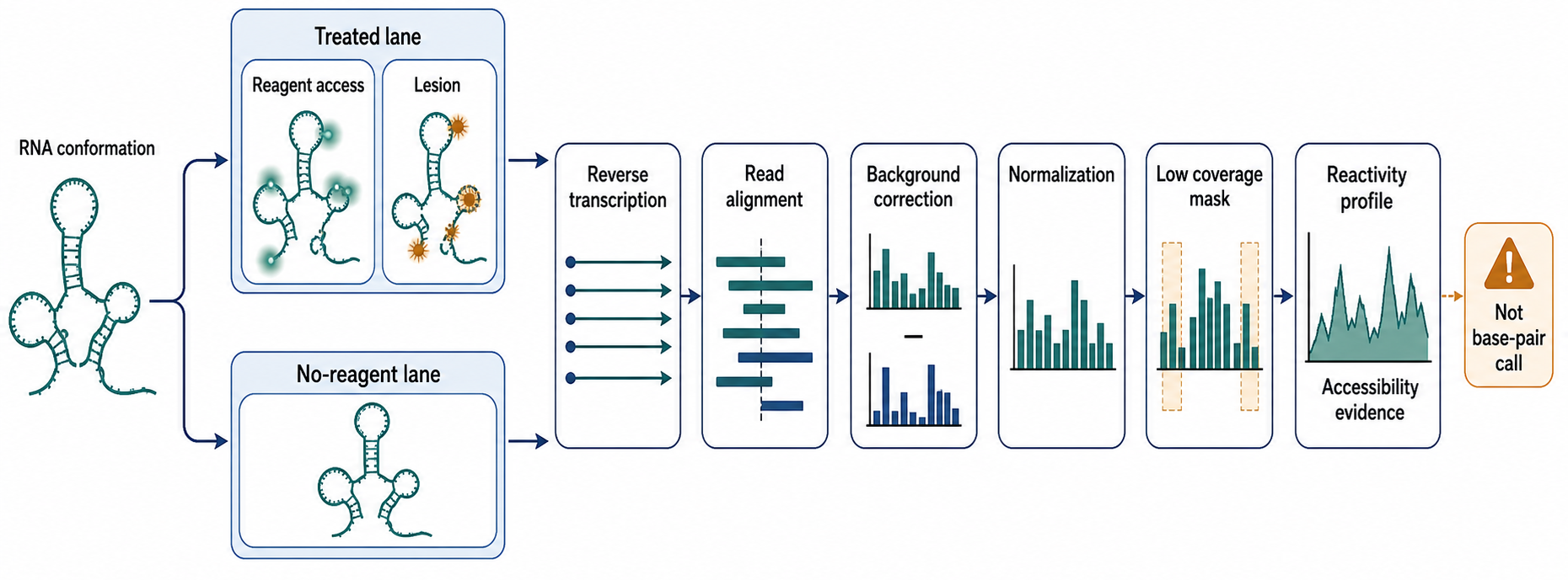
Figure 131.1. From RNA Reaction to Reactivity Measurement. A causal workflow follows sample definition, reagent reaction, quenching, extraction, reverse transcription, library construction, sequencing, alignment, event counting, control correction, normalization, uncertainty, and quality flags. The endpoint is a measurement track rather than a structure.
Selective 2′ hydroxyl acylation analyzed by mutational profiling, or SHAPE-MaP, is a foundational example of this evidence chain. SHAPE reagents react with the ribose 2′ hydroxyl when local backbone geometry and dynamics favor acylation. Flexible nucleotides tend to be more SHAPE-reactive, while nucleotides stabilized by base pairing, stacking, tertiary contacts, or protein protection tend to be less reactive. In SHAPE-MaP, reverse transcriptase reads through many SHAPE adducts and introduces mutations into cDNA rather than simply stopping. Sequencing those cDNAs makes it possible to estimate mutation rates at many positions and convert them into a reactivity profile.
The first-use definition matters because “SHAPE-reactive” is not equivalent to “single-stranded.” A nucleotide in a loop is often reactive because the ribose is flexible, but a nucleotide inside a helix can show signal if the helix breathes, if the local geometry is strained, or if the reactive group is transiently exposed. Conversely, a loop nucleotide can be low-reactive if it is stacked, ligand-bound, protein-protected, chemically modified, or poorly covered. SHAPE-MaP therefore measures local conformational behavior and access to a chemical reaction, not a binary state.
Box 131.1. Reactivity Is Evidence, Not a Base-Pair Label
The box separates the observed chemical event, corrected measurement, local accessibility interpretation, and downstream structural model. It directs model construction to Chapter 63.
Dimethyl sulfate mutational profiling with sequencing, or DMS-MaPseq, uses a different chemical window. DMS is a small methylating reagent that can enter many cellular contexts and modify accessible nucleobase atoms. Classical DMS structure probing emphasizes adenine and cytosine because DMS methylation of the Watson-Crick faces of those bases is strongly suppressed by canonical base pairing. In DMS-MaPseq, DMS-induced lesions are detected as reverse-transcription mutations after sequencing. The local references for this chapter include a practical DMS-MaPseq protocol for in vitro and cellular samples, an optimized rice implementation, and a recent mutation-signature filtering study that improves all-four-base DMS inference under defined conditions.
DMS-MaPseq is especially useful for in-cell probing because DMS is small, fast, and compatible with many biological samples. A bacterial culture, a mammalian cell line, or a plant tissue can be treated before RNA extraction, preserving some cellular context. Yet this advantage introduces new assumptions. Reagent concentration, exposure time, quenching, cell-wall or membrane access, tissue heterogeneity, viability, and stress responses can all affect the profile. In plant samples such as rice, protocol optimization is not a cosmetic detail; the physical properties of plant tissue can change reagent penetration, RNA extraction efficiency, and the background mutation spectrum.
In vivo click selective 2′ hydroxyl acylation and profiling experiment, or icSHAPE, adapts SHAPE-related chemistry to transcriptome-scale cellular analysis. The core idea is to use a clickable SHAPE reagent so that modified RNA fragments can be chemically tagged and enriched before sequencing. This enrichment helps recover signal from complex transcriptomes, where unmodified fragments and abundant RNAs would otherwise dominate. The method is conceptually close to SHAPE because it reports ribose flexibility, but it is experimentally different because it adds click chemistry, enrichment, and transcriptome-scale library construction.
Structure-seq is a DMS-based transcriptome-wide strategy, historically important for showing that in vivo RNA structural profiles could be surveyed across plant transcriptomes. The method treats living material with DMS, captures modified or stop-associated signals by sequencing, and maps those signals across many RNAs. Later refinements improved sensitivity, library construction, and analysis. Here, structure-seq and icSHAPE are compared at the level of chemistry, enrichment, library output, and measurement limitations; detailed historical priority claims are not made from the limited verified source set.
Table 131.1 compares the method families at the level a reader needs before interpreting a dataset. The important comparison is not a ranking. SHAPE-MaP, DMS-MaPseq, icSHAPE, and structure-seq ask related but nonidentical questions. SHAPE-family data can in principle report all four ribonucleotides through ribose chemistry. Classical DMS data emphasize accessible adenine and cytosine base faces. icSHAPE gains sensitivity through enrichment but inherits enrichment and abundance biases. Structure-seq made genome-wide in vivo DMS profiling practical in plant systems but depends strongly on tissue handling and mapping. The right method depends on the biological question, sample type, RNA abundance, required resolution, and acceptable perturbation.
Table 131.1. Probing Method Families and Raw Measurement Products. Chemical and enzymatic probing families convert different molecular events into mutations, stops, cleavage, or enrichment; exported reactivity is an assay-specific measurement rather than a direct structure.
| Family | Molecular event | Library/read feature | Primary exported measurement | Principal measurement limitation |
|---|---|---|---|---|
| SHAPE-MaP | Ribose 2′-hydroxyl acylation | Reverse-transcription mutations | Per-position event rate and normalized reactivity | Flexibility and access are not paired/unpaired labels |
| DMS-MaPseq | DMS methylation of accessible base atoms | Mutation signatures | Base-aware event rate and normalized contrast | Chemistry, reverse transcriptase, and classifier determine interpretable bases |
| icSHAPE | Clickable SHAPE-related reaction | Enriched modified fragments | Transcriptome-scale enrichment/reactivity signal | Enrichment and abundance alter library composition |
| Structure-seq | DMS reaction in intact material | Stop- or mutation-associated reads | Transcriptome-scale DMS profile | Penetration, tissue handling, mapping, and annotation matter |
| Enzymatic probing | Structure-biased cleavage or modification | Ends, truncations, or modified reads | Regional accessibility/cleavage profile | Enzyme sterics, sequence preference, salt, and kinetics |
| SHAPE-JuMP-like readout | Chemistry-linked jump event | Noncolinear cDNA feature | Sparse coordinate-pair constraint table | Template switching, chimeras, mapping, and coverage |
The first major evidence boundary is that all these methods average across molecules unless the design explicitly preserves molecule-level linkage. A treated mammalian mRNA library may contain nascent transcripts, mature cytoplasmic mRNAs, translating mRNAs, decay intermediates, isoforms with different untranslated regions, and protein-bound subpopulations. A single reactivity value at one nucleotide can therefore represent a mixture. Intermediate reactivity may mean that every molecule is moderately flexible, or that half the molecules are strongly protected and half are strongly exposed. Most short-read mutational profiling cannot distinguish those cases without additional design.
The second evidence boundary is that a probing experiment measures the sample as prepared. In vitro refolding can reveal sequence-intrinsic folding under chosen salt, temperature, and magnesium conditions, but it lacks co-transcriptional folding, RNA-binding proteins, translation, cellular crowding, and native RNA modification patterns unless these are deliberately included. In-cell probing includes biological context, but the cell is not an inert vessel. Treatment can induce stress, change RNA localization, alter translation, or bias recovery of fragile transcripts. A mature interpretation often compares in vitro, lysate, and in-cell profiles rather than treating one condition as the sole truth.
A concrete example is a viral RNA genome. In vitro probing can show which elements fold from sequence alone. In infected cells, the same genome may be translated by ribosomes, copied by a viral polymerase, packaged into virions, protected by nucleocapsid proteins, recognized by innate immune factors, or sequestered in replication compartments. A difference between in vitro and in-cell DMS-MaPseq profiles might reflect a protein-bound packaging signal, a long-range RNA-RNA interaction, ribosome transit, or a change in which viral RNA species dominate the library. The profile is valuable precisely because it exposes these possibilities, but it does not choose among them without additional evidence.
The verified source set supports recent DMS-MaPseq practice, optimized plant DMS-MaPseq, DMS mutation-signature filtering, web-based analysis, and viral RNA probing review synthesis. Claims about other method families are kept to the measurement principles needed for comparison and do not assert unsupported historical or performance rankings.
131.2. SHAPE-JuMP and long-range structural readouts
Standard reactivity profiles are local. They report whether individual nucleotides reacted more or less under a condition, but they usually do not identify which distant nucleotides were near each other in the folded RNA. This is a serious limitation because many biologically important RNA structures depend on long-range organization. Viral genomes can pair distant untranslated regions with coding-region elements. Riboswitches bring helices together around ligand-binding pockets. Introns and repeats can pair over long distances to affect splicing or circular RNA formation. Long noncoding RNAs may contain modular domains separated by thousands of nucleotides.
SHAPE-JuMP addresses part of this limitation by converting some SHAPE-associated events into cDNA-encoded jumps. In simplified terms, a reverse transcriptase encountering a SHAPE-induced lesion or crosslink-like event can produce a cDNA molecule that joins sequence positions that were proximal in the RNA population. Computational analysis then searches for these noncolinear or jump-like read features and filters them against background. The resulting signal is a proximity-like constraint. It does not provide a complete three-dimensional contact map, and it does not have the same physical meaning as an RNA-RNA proximity ligation experiment, but it can add long-range information that local reactivity lacks.
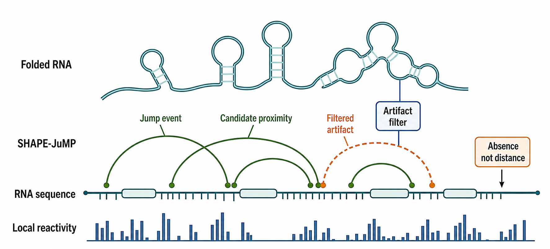
Figure 131.2. Local Profiles and Pairwise Jump Measurements. Parallel panels contrast a one-dimensional per-nucleotide reactivity profile with sparse pairwise SHAPE-JuMP-like event records. Each panel displays raw event counts, eligible coverage, background, normalized value, and missingness so the different measurement geometries remain explicit.
The distinction between local reactivity and long-range proximity is pedagogically important. Imagine a viral 5′ untranslated region and a downstream coding-region element. A SHAPE profile provides separate values along both regions. A SHAPE-JuMP-like library can additionally yield reads linking coordinate pairs, producing a sparse pairwise count table rather than a one-dimensional track. If no jump is observed, the absence does not prove the regions never approach. Low coverage, inefficient lesion formation, reverse-transcription bias, filtering thresholds, or transient proximity can all erase a true event from the detected dataset.
Long-range readouts require stronger measurement accounting than a simple contact-like heat map suggests. Each pair should preserve raw event count, eligible coverage, background count, replicate support, mapping uniqueness, normalized score, uncertainty, and quality flags. If a signal overlaps an RNA-binding-protein site, the sample metadata should record the relevant RNP condition because the event may arise from RNA geometry, protein-mediated juxtaposition, or a mixed population. Deciding among those structural explanations belongs to Chapter 63.
The main artifact class is template switching or chimeric library formation. Reverse transcriptases can jump for reasons unrelated to true RNA proximity. Library preparation can create chimeras. Repetitive sequences can map ambiguously. Highly abundant RNAs can generate rare artifactual links that look convincing because the read count is high. A reproducible jump across biological replicates is more persuasive than a single high-count event in one library. A jump that disappears in a no-reagent control, appears at plausible positions, and agrees with local reactivity or mutational evidence is stronger than a jump that only passes a read-count threshold.
SHAPE-JuMP also illustrates a broader principle: more dimensional data are not automatically more certain data. A two-dimensional matrix feels visually closer to a structure than a one-dimensional profile, but each matrix entry still has a readout model. Analysts must know what event produced the signal, what background was subtracted, what filtering was applied, and what false-positive modes remain. The measurement-layer product is therefore a sparse interaction-constraint export with explicit missingness, not a solved contact map.
Boundary cases are common. A compactly folded tRNA has many true proximal positions, but chemical modification and reverse transcription through tRNA modifications can be difficult. A long lncRNA may show sparse long-range signals because coverage is poor, not because the molecule is unstructured. A viral genome may produce many contacts because it exists in several functional states; a population-average contact map may blend translation, replication, and packaging conformations. In all three cases, long-range structural readouts are useful only when the molecular population is defined.
131.3. Enzymatic probing, in-cell probing, and transcriptome-wide reactivity
Enzymatic probing predates sequencing-coupled structuromics and remains useful because enzymes can discriminate broad structural features. A single-strand-preferring nuclease can cut flexible or unpaired regions. A double-strand-preferring nuclease can enrich for helical regions. Other enzymatic or protein-mediated readouts can favor accessible loops, duplexes, or specific structural contexts. In older experiments, cleavage products were often resolved by gels or primer extension. In high-throughput formats, cleavage, truncation, or modified ends can be encoded by sequencing.
The mechanistic bridge is that an enzyme is not a small chemical reagent. DMS is small enough to access many narrow molecular spaces. A nuclease is a folded protein with a binding surface, catalytic geometry, sequence preferences, and salt requirements. Therefore enzymatic cleavage is a compound signal: the RNA must present a compatible structural feature, the enzyme must physically access the site, the sequence context must be acceptable, and the reaction must occur before the RNA or complex changes state. A missing enzymatic cut does not necessarily mean a nucleotide is base-paired. It can mean steric occlusion by a protein, unfavorable local sequence, poor enzyme kinetics, or protection by tertiary packing.
Enzymatic probing is strongest when the experimental question matches this measurement window. If the goal is to distinguish broad single-stranded and double-stranded regions in a purified RNA, nuclease panels can be informative. If the goal is to measure nucleotide-resolution flexibility inside dense RNPs, small-molecule probing is usually less confounded by steric access. If both chemical and enzymatic probes agree, confidence increases. If they disagree, the disagreement can be informative: a site that is chemically reactive but nuclease-resistant may be small-molecule accessible yet sterically shielded from proteins, whereas a nuclease-sensitive site with modest chemical reactivity may reflect enzyme recognition of a longer flexible region.
In-cell probing asks how RNA behaves in a biological context. The term means that the reagent is applied before RNA extraction, while cells, tissues, virions, or organisms remain intact enough to preserve relevant molecular states. In-cell probing is valuable because cellular RNA is not simply naked RNA. Proteins bind it, ribosomes translocate along it, helicases remodel it, metabolites stabilize or destabilize domains, ions alter folding, RNA modifications change base pairing and reverse transcription, and compartments impose different chemical environments. The cellular profile can therefore reveal the structural state that a transcript experiences in function.
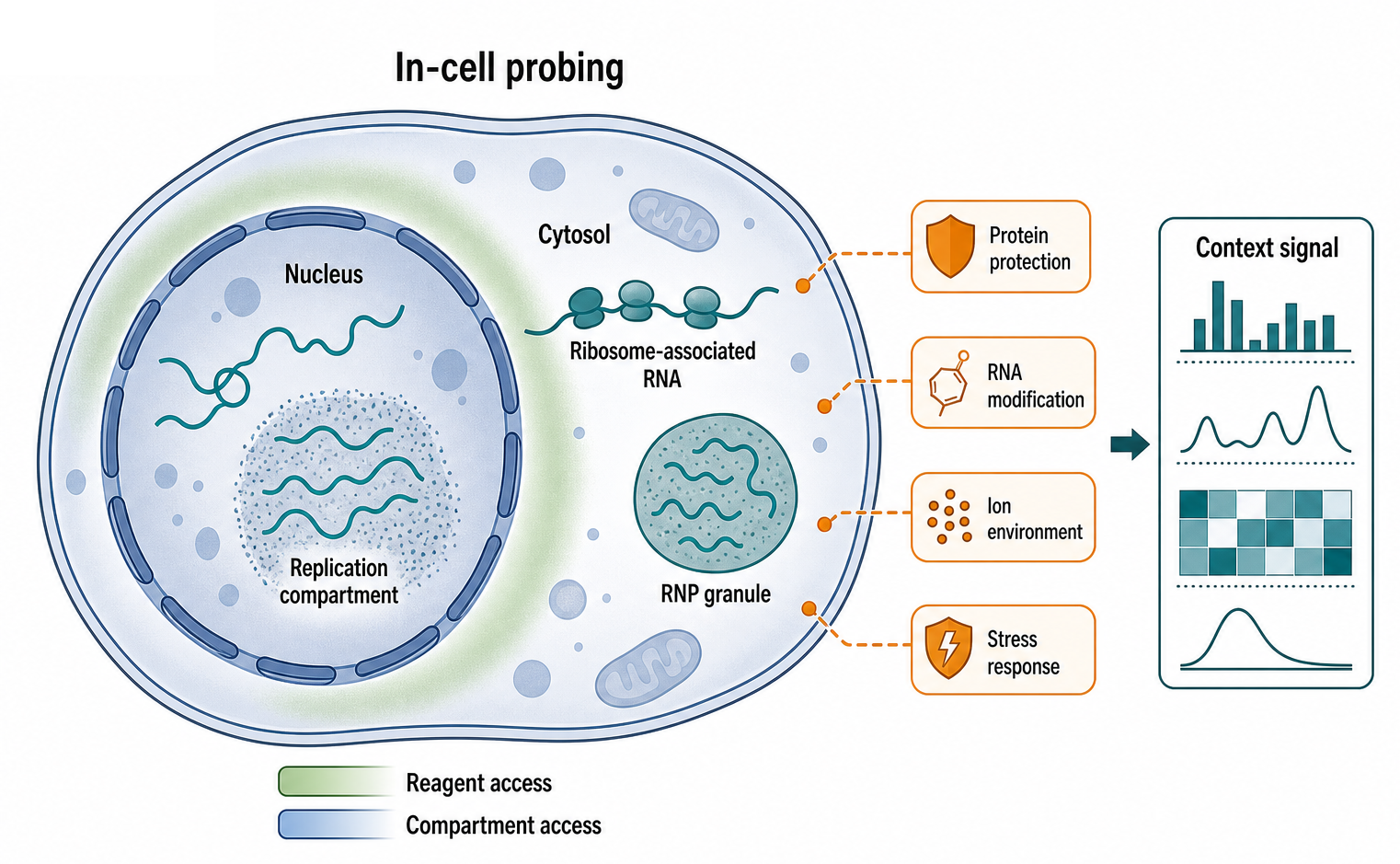
Figure 131.3. Sample Context Defines the Measured RNA Population. Purified RNA, lysate, cultured cells, tissues, virions, and delivered synthetic RNA are shown as distinct conditions. The figure traces how penetration, viability, compartment, isoform composition, RNP occupancy, extraction, and enrichment determine which molecules enter the library.
The same realism creates confounders. A decrease in DMS reactivity in cells compared with in vitro RNA may indicate base pairing in the cell. It may also indicate protein binding, ribosome protection, methylation of the target base, poor reagent access to a compartment, a shorter isoform lacking the mapped region, or RNA degradation after treatment. An increase in SHAPE reactivity in cells may indicate unfolding by a helicase or ribosome, but it may also reflect stress-induced transcript remodeling or different ionic conditions. A careful chapter reader should ask: what exactly changed, and how was each alternative controlled?
Box 131.2. Define the Measured Molecular Population
A checklist asks whether the library represents nascent, mature, translating, packaged, replicating, degraded, purified, formulated, or delivered RNA and records mixtures explicitly.
Transcriptome-wide reactivity is a large-scale version of the same measurement. A total RNA or enriched RNA population is probed, converted to sequencing libraries, and mapped across many transcripts. This can expose broad patterns, such as structured untranslated regions, accessible translation-initiation regions, differences between coding and noncoding regions, or stress-dependent remodeling. It can also expose gene-specific hypotheses: a candidate riboswitch-like element, a viral frameshift region, a structured 3′ untranslated region, or a lncRNA domain worth targeted validation.
The phrase “transcriptome-wide” is often overread. It means the assay was capable of surveying many transcripts, not that every transcript was measured well. Low-abundance transcripts may have no reliable per-nucleotide data. Isoforms sharing exons may be impossible to separate with short reads. Repetitive elements, paralogous genes, duplicated viral sequences, organellar transcripts, and rRNA fragments can create ambiguous alignments. Highly abundant rRNAs and tRNAs can dominate unless depleted or separately analyzed. A transcriptome-wide figure should always be accompanied by coverage thresholds, masking rules, and transcript-model assumptions.
Table 131.2 summarizes biological contexts and the main interpretation hazards. Bacterial mRNAs bring operon structure, co-transcriptional folding, translation-coupled remodeling, and riboswitch logic. Plant tissues bring cell walls, organelles, tissue mixtures, and stress physiology; optimized DMS-MaPseq in rice is a useful local reference for organism-specific tuning. Viral RNAs bring compact genomes with dense functional structures, but the same RNA molecule can serve as genome, mRNA, replication template, packaging substrate, and immune ligand. Mammalian transcriptomes bring isoform diversity, compartmentalization, RNA-binding proteins, and extensive regulatory RNP states. Synthetic RNAs bring controlled sequence and manufacturing history, but their relevant structure may differ before and after cellular delivery.
Table 131.2. Biological Contexts and Measurement Hazards. In vitro, cellular, tissue, low-input, and heterogeneous probing contexts define different RNA populations and artifact risks; interpretation requires metadata for abundance, treatment, compartment, and sample handling.
| Context | Population that must be defined | Characteristic hazard | Required metadata |
|---|---|---|---|
| Bacterial RNA | Growth phase, operon, translation state | Rapid stress and cotranscriptional remodeling | Strain, growth, timing, dose, quench |
| Plant tissue | Tissue, developmental stage, organelles | Penetration and heterogeneous cell states | Tissue, stage, penetration, organellar mapping |
| Viral RNA | Genome, transcript, replication, or packaging state | Mixed species and subgenomic ambiguity | Infection stage, enrichment, strand/species rules |
| Mammalian transcriptome | Cell type, compartment, isoform, RNP state | Shared exons and low-abundance dropout | Cell state, fractionation, annotation, selection |
| Stable RNA controls | Mature versus precursor rRNA/tRNA | Natural modifications and extreme abundance | Depletion, mapping, modification-aware handling |
| Synthetic RNA | Purified, formulated, delivered, or translating population | Manufacturing and delivery change the state | Sequence, chemistry, formulation, dose, time |
A concrete in-cell example is a synthetic mRNA delivered for expression. In vitro probing of the purified RNA may reveal stable coding-region helices, accessible UTR elements, or structures near the cap and poly(A) tail. After delivery into cells, the same RNA may associate with cap-binding proteins, initiation factors, ribosomes, helicases, decay enzymes, and innate immune sensors. Chemical modifications used to tune immunogenicity or translation can also alter folding and reverse transcription. If the question is manufacturing quality, in vitro probing may be appropriate. If the question is intracellular translation, in-cell or lysate probing may be more relevant.
Another example is a bacterial riboswitch. A ligand-free riboswitch may expose an expression platform, while ligand binding stabilizes an aptamer and changes downstream base pairing. A DMS or SHAPE profile can identify nucleotides that become protected or exposed upon ligand addition. The evidence becomes mechanistic when the differential profile aligns with a known aptamer architecture, when ligand concentration dependence is observed, when mutations disrupt the predicted pair, and when compensatory mutations restore regulation. Without those checks, a reactivity change is a candidate mechanism, not proof of regulatory causality.
For viral RNAs, a review anchor in the local references emphasizes that chemical and enzymatic probing has matured from targeted mapping to higher-throughput and in-cell analysis. Viral systems remain difficult because population heterogeneity is biologically meaningful. An infected-cell profile may contain newly synthesized genomes, translating genomes, replication intermediates, packaged RNA, defective RNAs, and host-bound viral RNAs. Strong viral RNA structure claims therefore state the infection stage, enrichment strategy, mapping approach, and whether the measured RNA population corresponds to the functional state being discussed.
131.4. Mutational readout generation, raw counts, and normalization
Mutational profiling is not just a convenient sequencing trick; it is the measurement model that connects chemistry to numbers. The raw observation is a collection of aligned reads. At a position, the analyst counts substitutions, deletions, insertions, stops, or other signatures depending on the protocol. The treated sample has a mutation rate. The no-reagent or mock-treated control has a background rate caused by reverse-transcription errors, RNA damage, sequencing errors, natural modifications, mapping errors, and sample handling. Reactivity is inferred from the difference, ratio, or modeled contrast between those rates after quality filtering.
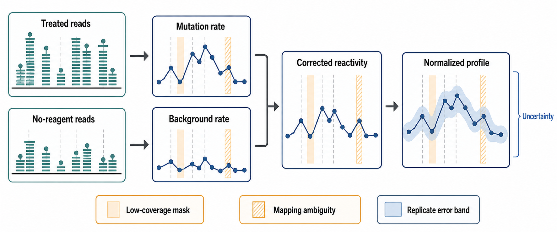
Figure 131.4. Mutational Readout Generation and Normalization. At one coordinate, treated and control reads generate event numerators and coverage denominators. The figure then shows background correction, filtering, normalization, uncertainty estimation, and missingness assignment, with branches for low coverage and high background.
The simplest conceptual formula is treated signal minus background. Real analysis is more complicated. Positions with low coverage cannot be trusted because a few reads can dominate the estimate. Positions in homopolymers, repeats, or paralogous regions can misalign. Natural RNA modifications can cause reverse-transcription mutations independent of the probing reagent. Damaged RNA can elevate background. PCR duplication can inflate confidence. Different reverse transcriptases have different read-through and error profiles. Sequencing platforms have base-quality patterns. These factors mean that mutation-rate estimation and filtering are part of the experiment, not downstream bookkeeping.
Normalization converts corrected signals into values that can be compared within a transcript or across related samples. Some pipelines use percentile-based scaling, excluding the most reactive outliers and scaling to a reference distribution. Others use denatured controls, spike-ins, replicate-aware models, or method-specific transformations. Normalization can change which nucleotides appear strongly reactive and can alter folding constraints. Therefore a published reactivity profile is incomplete without the normalization method and masking rules.
The most common interpretive error is to compare profiles normalized by incompatible pipelines as though they were absolute measurements. A SHAPE profile normalized within a purified RNA cannot be directly compared with a DMS profile normalized across a transcriptome. Even two DMS-MaPseq datasets can differ if one uses mutation-signature filtering, different coverage thresholds, or a different transcript annotation. Comparative claims should be made within a matched design whenever possible: same reagent, similar treatment, shared library strategy, same mapping reference, same normalization, and replicate-aware statistics.
Box 131.3. Before Comparing Reactivity Profiles
A matched-design checklist covers reagent, dose, exposure, quenching, extraction, reverse transcriptase, library, read length, reference, controls, coverage, masks, normalization, replicates, and alternative causes of differential signal.
Mutation-signature filtering is a recent example of the readout model becoming more sophisticated. The local Mitchell et al. reference reports that filtering mutation signatures can enable high-fidelity DMS probing at all four nucleobases. The conceptual advance is that the pattern of mutations, not just their total rate, can help distinguish reagent-induced lesions from background. This is powerful but also makes the computational classifier part of the assay. The method should not be generalized to every DMS dataset unless the chemistry, reverse-transcription conditions, sequencing depth, and filtering assumptions match the validated setting.
Differential reactivity analysis compares profiles between conditions. Examples include ligand versus no ligand, infected versus uninfected cells, wild type versus protein knockout, heat shock versus control, or in vitro versus in-cell RNA. A statistically supported change means the measured reactivity changed. It does not automatically mean that the RNA folded differently. The change can arise from altered protein occupancy, abundance, isoform usage, RNA modification, compartment access, degradation, sequence composition, or technical variation. Replicate-aware analysis can reduce false positives, but biological interpretation still requires a model of what changed in the sample.
Table 131.3 presents common analysis quantities and their failure modes. Treated mutation rate is sensitive to lesion chemistry and reverse-transcription behavior. Background rate is sensitive to RNA damage and natural modifications. Corrected reactivity is sensitive to subtraction model and low coverage. Normalized reactivity is sensitive to scaling choice. Differential reactivity is sensitive to replicate variance and compositional changes. Contact-like jump counts are sensitive to template switching and mapping. A transparent analysis report should expose each of these quantities rather than only the final color-coded structure.
Table 131.3. Measurement Quantities, Failure Modes, and Export Fields. Mutation rate, stop rate, cleavage, enrichment, normalized reactivity, and model-derived constraints use different numerators, denominators, and failure modes; reusable exports must preserve the underlying measurement definition.
| Quantity | Numerator/denominator or model | Common failure mode | Required export field |
|---|---|---|---|
| Treated event rate | Treated events / informative coverage | RT, sequence, quality, duplication, mapping bias | Treated count and coverage |
| Control background | Control events / informative coverage | Damage, modifications, or mismatched handling | Control count and coverage |
| Corrected value | Declared treated-control contrast | Unstable low-count subtraction | Correction formula and uncertainty |
| Normalized reactivity | Declared scaling transformation | Outliers or incompatible scaling sets | Normalization method and scope |
| Differential reactivity | Replicate-aware condition contrast | Abundance, isoform, access, or batch shifts | Effect, variance, replicates, flags |
| Pairwise jump score | Filtered pair events against background | Chimeras, repeats, sparse coverage | Coordinates, counts, score, uncertainty |
| Missing value | No valid quantitative estimate | Missing silently encoded as zero | Missing flag and reason code |
A practical example shows why normalization matters. Suppose a riboswitch aptamer has one highly reactive linker and many moderately reactive loop residues. If normalization scales by the top percentile, the linker may compress the apparent signal of the loops. If an outlier-clipping method removes the linker, the loops may appear more reactive. If ligand binding protects the linker, the normalization distribution changes again. A naive before-and-after plot can therefore create apparent global changes from a local shift. The correct analysis reports raw mutation rates, background, normalized values, replicate variance, and the effect of the normalization choice.
Another example is a low-abundance lncRNA. A transcriptome-wide dataset may produce sparse reads across the locus. Low mutation counts in a region might look like protection, but the position may simply lack coverage. If reads map equally well to several isoforms, a putative structural domain may be assigned to the wrong transcript. Targeted amplicon probing, capture enrichment, long-read-informed annotation, or orthogonal validation may be required before claiming a lncRNA structural feature.
The readout model also matters for RNA modifications. Modified bases can alter reverse-transcription behavior, chemical reactivity, and mapping. A naturally modified adenosine that causes misincorporation may elevate background in the no-reagent control. A modification that blocks DMS methylation may reduce treated signal. A modified region that affects folding may produce a real structural difference and a detection artifact at the same time. For this reason, chapters on RNA modification detection and direct RNA sequencing provide important cross-context for interpreting unusual mutational profiles.
131.5. Measurement outputs, reactivity profiles, and constraint-data export
The endpoint of this chapter is a measurement product that another analyst can inspect without rerunning the entire experiment. For local probes, the main processed output is an ordered reactivity profile tied to a specific reference sequence and coordinate system. For SHAPE-JuMP or related long-range readouts, the output can be a table of ordered coordinate pairs with event counts, background estimates, normalized interaction scores, uncertainty, and filtering status. Neither representation is a structure. Each is a constraint-ready measurement with an explicit physical origin.
Sequence identity is part of the measurement. An export should include the exact RNA sequence or a checksum and stable reference identifier, reference version, transcript or isoform identifier, coordinate origin, strand, and any sequence edits used in the construct. For amplicons, primer-derived or unmeasured terminal regions should be marked. For viral and organellar RNAs, strand and genome version are essential. For transcriptome-wide data, genomic and transcript coordinates should not be mixed without a declared mapping.
Reactivity records need both values and provenance. Each position should preserve treated event count, treated coverage, control event count, control coverage, corrected value, normalized reactivity, uncertainty, and quality status when those quantities exist. A profile containing only final normalized values prevents users from distinguishing a well-measured low-reactivity position from a low-coverage or high-background position that happened to receive the same number. Raw or minimally processed count tables should therefore remain linked to the normalized export.
Missingness is not zero. A nucleotide can be missing because no reads cover it, coverage falls below threshold, mapping is ambiguous, background is excessive, a primer or adapter masks it, the transcript isoform lacks the coordinate, or a quality rule excludes it. These causes have different implications. A versioned export should encode missing values explicitly and attach a reason code rather than replacing them with zero reactivity.
Uncertainty can be represented as a standard error, confidence or credible interval, replicate variance, bootstrap interval, or method-specific score. The representation must state what source of variation it includes. Technical counting uncertainty does not capture biological variation, and replicate variance does not automatically capture mapping or normalization bias. When uncertainty cannot be estimated, the export should say so instead of implying exactness.
A practical versioned handoff object has the following logical structure:
schema: rnabook.probing_measurement.v1
target:
 sequence_id: stable identifier or checksum
 sequence: exact assayed sequence or declared external reference
 coordinate_system: transcript, genome, amplicon, or construct coordinates
measurement:
 profile: position, base, treated_count, control_count, coverage, corrected_value, normalized_reactivity, uncertainty
 interaction_constraints: position_i, position_j, raw_count, background, normalized_score, uncertainty
quality:
 missingness: per-position missing flag and reason
 flags: low_coverage, high_background, ambiguous_mapping, replicate_discordance, saturation, or protocol-specific flags
metadata:
 sample, condition, reagent, dose, exposure, quench, extraction, reverse_transcriptase, library, sequencing, mapping, normalization, replicate
caveats:
 free-text and controlled statements limiting comparison or interpretation
The schema version should change when field meaning changes, not whenever a value is updated. A data release can have its own object version, checksum, generation timestamp, software and parameter record, and parent-object identifier. This distinction supports provenance: v1 defines field semantics, while a release identifier distinguishes corrected mapping, revised masks, or recalculated normalization.
Profile exports and interaction-constraint exports should share metadata and quality conventions but need not be forced into one rectangular table. Per-nucleotide profiles are naturally one-dimensional. Long-range constraints are sparse pairwise records. Both should reference the same assayed sequence, sample, condition, and replicate definitions so a consumer can determine whether the data are comparable.
Constraint-data export also requires units and scale semantics. A normalized SHAPE value, DMS mutation-rate contrast, enzymatic cleavage enrichment, and jump score are not interchangeable. Each field should name its measurement type, transformation, normalization scope, expected range if bounded, and whether larger values mean greater reaction, cleavage, or support for a pairwise event. Cross-study harmonization must not erase these distinctions.
Chapter 63 consumes the versioned handoff object to perform structural inference. That chapter decides how to convert reactivities or interaction constraints into algorithmic terms, compare inferred models with benchmarks, propagate measurement uncertainty into structural uncertainty, and detect overfitting. The handoff boundary protects both layers: model revisions do not rewrite the archived measurement, and measurement corrections can be traced to the models that consumed them.
131.6. Controls, artifacts, measurement benchmarks, and reproducibility
Controls are not peripheral in high-throughput RNA structure probing; they define the measurement. The minimal design includes a treated sample and a no-reagent or mock-treated control processed through the same extraction, reverse-transcription, library, sequencing, and mapping pipeline. Biological replicates are needed when the goal is biological inference rather than method demonstration. Coverage thresholds are needed because low-read positions cannot support nucleotide-resolution claims. The analysis must report how positions were masked, how background was corrected, how reactivity was normalized, and which transcript annotation was used.
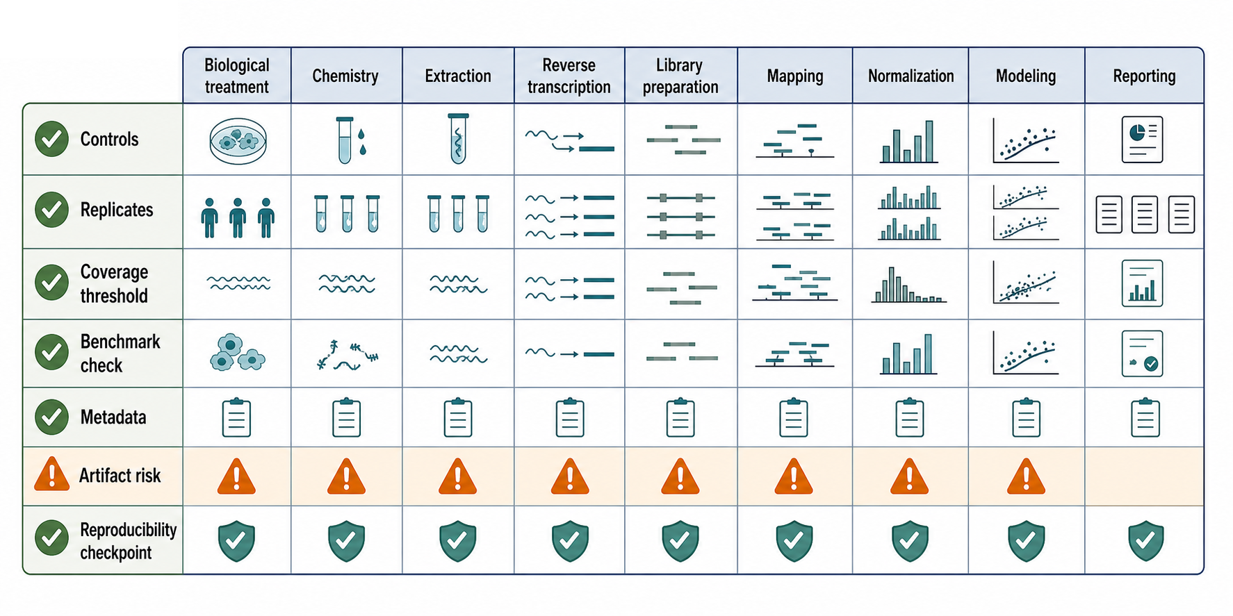
Figure 131.6. Measurement Quality and Reproducible Export Gates. A gate diagram moves from treatment controls through molecular controls, library and mapping controls, replicate checks, measurement benchmarks, and reproducible regeneration. The final gate emits rnabook.probing_measurement.v1 with sequence, coordinates, profiles or interaction constraints, uncertainty, coverage, metadata, flags, and caveats for Chapter 63.
Treatment controls address whether the reagent measured the intended state. For in-cell DMS or SHAPE-related probing, the investigator should consider reagent dose, exposure duration, quenching, cell viability, stress induction, and sample penetration. A reagent that kills cells or triggers a strong stress response may measure a perturbed state rather than the intended physiology. For tissues, penetration may differ by cell type. For viruses, treatment stage and enrichment strategy determine whether the measured RNA represents virions, infected cells, replication complexes, or mixed states.
Molecular controls address whether chemistry behaved as expected. No-reagent controls estimate background mutation or stop rates. Denatured controls can help identify chemically accessible positions under unfolded conditions, although denatured controls are not always biologically relevant. Spike-ins can monitor reaction and library efficiency if they are chosen carefully. Known-structure RNAs such as rRNA elements, tRNAs, or synthetic controls can reveal gross chemistry or analysis failures, but they are not perfect internal standards because modifications, abundance, and RNP context differ.
Library and mapping controls address whether sequencing counts represent molecules accurately. Reverse transcriptase choice, read length, PCR duplication, base quality, adapter trimming, and aligner parameters all matter. Reads from repetitive elements, paralogs, organelles, viral subgenomic RNAs, and shared exons can map ambiguously. If the experiment uses amplicons, primer binding can bias coverage and exclude isoforms. If the experiment uses poly(A) selection, nonpolyadenylated RNAs and decay fragments are missed. If it uses rRNA depletion, depletion efficiency changes library composition.
Normalization and statistical controls address whether the final profile supports the stated comparison. Replicate concordance should be assessed before differential claims. Differential reactivity should be modeled with variance, not inferred from one treated-control subtraction. Outlier clipping, percentile scaling, and coverage masking should be reported. Comparing profiles from different studies requires harmonized metadata: organism, cell type, reagent, dose, treatment duration, extraction, library type, read length, mapping reference, normalization, and replicate design. Repositories and web platforms can support reuse, but reuse is only as strong as the accompanying metadata.
Measurement benchmarking asks whether chemistry, library construction, counting, correction, normalization, and filtering recover known inputs and reject known artifacts. Synthetic RNAs can test reagent response and sequence context; mixtures with known proportions can test linearity and dynamic range; matched technical replicates can test precision; negative controls can estimate false event rates. Long-range readouts should be challenged with chimeric-library and ambiguous-mapping controls. All-four-base DMS pipelines should test whether mutation-signature classification generalizes across the chemistry and reverse-transcription conditions for which the measurement is claimed. Benchmarking inferred structures remains in Chapter 63.
Reproducibility has several layers. Technical reproducibility means the same sample and protocol produce similar raw and normalized measurements. Biological reproducibility means independent biological samples show consistent profiles or contrasts. Analytical reproducibility means the same raw reads, references, parameters, and code regenerate the same counts, masks, reactivities, interaction constraints, and handoff object. A chapter or paper should provide raw and processed data, reference versions, parameters, scripts or workflow descriptions, checksums, and enough metadata to rerun the measurement layer. Web-based platforms can improve accessibility, but durable reproducibility still requires transparent inputs and outputs.
Scientific cautions should be stated plainly. DMS reactivity does not simply equal single-stranded RNA. SHAPE reactivity does not simply equal unpaired RNA. An in-cell profile should not be called “the native structure” without specifying molecular population and condition. Transcriptome-wide does not mean complete coverage. Missing signal is not zero reactivity. A no-signal region should not be interpreted without checking coverage and background. Normalized profiles from incompatible pipelines should not be compared as absolute quantities. Structural conclusions from these measurements belong to Chapter 63.
Recent Consensus
Consensus in the field is converging on a disciplined measurement view. SHAPE and DMS are complementary chemistries. Enzymatic probing remains useful when steric and sequence biases are reported. In-cell probing adds biological context but requires treatment and sample controls. Long-range readouts add pairwise constraint measurements but require stringent artifact filtering. Reusable releases preserve raw counts, normalized outputs, uncertainty, missingness, metadata, quality flags, and caveats rather than publishing only a colored reactivity track.
Open Questions, Controversies, Deprecated Models, and Common Misconceptions
Open questions:
- How can population-average measurements preserve enough molecule-level linkage for later ensemble inference?
- How can short-read probing be integrated with long-read or single-molecule measurements without conflating assay scales?
- Which uncertainty models best separate counting, replicate, mapping, and normalization uncertainty?
- How can datasets from different reagents, organisms, and pipelines be normalized for cross-study synthesis?
- Which measurement benchmarks and reference materials should be required before a new probing chemistry or analysis pipeline is treated as generally reliable?