Chapter 63. Inference from RNA Probing and Interaction Constraints to Structural Models
Scope Note
This chapter explains how normalized RNA probing and interaction-constraint data objects become secondary-structure, ensemble, and integrative structural models. It owns constraint encoding, reactivity-to-model transformations, multi-condition and transcriptome-scale inference, integration of RNA-RNA and RNA-protein constraints, model benchmarking, uncertainty, and overfitting. Probing chemistry, sample and library preparation, raw counts, normalization, controls, measurement artifacts, assay benchmarks, and constraint-data export belong to Chapter 131. Thermodynamic and ensemble foundations are treated in Chapters 60 and 61, and comparative inference in Chapter 62.
Executive Summary
Structural inference begins from a versioned constraint-data object, not from a raw sequencing library. The object identifies the sequence and coordinate system; provides normalized per-nucleotide reactivities or interaction constraints; carries uncertainty or confidence fields; distinguishes missing values through coverage masks; records condition and replicate metadata; and retains control-derived quality flags, normalization provenance, and assay-specific caveats. Chapter 131 produces and validates this object. This chapter interprets it under an explicit structural model.
Probing-constrained modeling maps normalized values and their uncertainty into folding scores, priors, or likelihood terms. A common secondary-structure use is a soft constraint: the algorithm changes the effective score of structural states so that high reactivity disfavors pairing and low reactivity can favor pairing, without forcing every nucleotide into one state. SHAPE-directed folding, probabilistic data-directed folding, and related methods can improve prediction when the handoff data are informative and the model matches the molecular state, but the constraints do not eliminate thermodynamic, comparative, and structural reasoning.
Transcriptome-wide and multi-condition probing expand the question from “What is the fold of this RNA?” to “Which regions change accessibility across cell states, proteins, isoforms, compartments, modifications, or time?” In that setting, a single minimum-free-energy model is often less informative than reactivity changes, ensemble shifts, differential structure scores, and carefully controlled comparisons. Long-read approaches such as Nano-DMS-MaP can connect structural information to isoforms, while co-transcriptional, single-cell, and nanopore methods begin to resolve heterogeneity that ensemble short-read profiles average away.
Integrative RNA structure modeling combines chemical probing with other constraints. RNA-RNA interaction maps can identify distant partners or intermolecular contacts that are invisible to one-dimensional reactivity alone. RNA-protein interaction maps can identify binding sites where low or high reactivity may reflect an RNP state rather than RNA-intrinsic base pairing. Comparative covariation, high-resolution structural data, biochemical mutagenesis, reporter assays, and genetic rescue experiments provide independent evidence needed to decide whether a proposed model is a functional structure, a transient ensemble member, a protein-protected region, or a processing artifact.
The central caution is that probing data should constrain a model, not replace scientific judgment. Failure modes include overfitting noisy reactivities, treating chemical accessibility as base-pair status, ignoring alternative conformations, normalizing incompatible experiments together, missing structured regions because proteins block reagent access, inferring RNA-RNA contacts from proximity without validating base-pairing, and benchmarking against training-like RNAs. A defensible model reports uncertainty, shows which data support which features, tests sensitivity to constraint strength, and validates important claims against independent evidence.
Concept Inventory
- RNA structure probing: the experimental measurement of nucleotide-level or region-level chemical reactivity, nuclease sensitivity, crosslinking, proximity, or mutational signature that reports some aspect of RNA conformation or RNP organization. In this chapter, “probing” mainly refers to chemical methods that modify accessible or flexible nucleotides and then read out the modified positions by reverse transcription, sequencing, or related assays.
- Constraint: information supplied to a folding model. A hard constraint forbids or requires specified structural states, such as “nucleotide 32 cannot pair” or “nucleotides 10 and 40 must pair.” A soft constraint changes the score of candidate structures without making a state impossible. Most chemical probing data are better treated as soft constraints because a reactive nucleotide can occasionally be paired, a protected nucleotide can be unpaired for reasons other than base pairing, and bulk experiments average over molecular ensembles.
- Pseudo-free-energy term: an empirical energetic bonus or penalty added to an RNA folding algorithm to make predicted structures more consistent with probing data. The term is not a physical free energy measured by calorimetry. It is a calibrated mapping from reactivity to score, usually designed so that high SHAPE reactivity disfavors pairing and low SHAPE reactivity modestly favors pairing. Pseudo-free-energy terms connect experimental data to dynamic programming algorithms introduced in Chapters 60 and 61.
- Reactivity profile: the processed vector of nucleotide-level values produced by a probing experiment. It may represent SHAPE adduct frequency, DMS mutation rate, icSHAPE signal, or another signal after background subtraction, normalization, and quality filtering. A reactivity profile is not a structure. It is a measurement layer that can be compared with a structure model.
- Mutational profiling: a readout strategy in which reverse transcriptase reads through certain chemical adducts and incorporates non-templated mutations at modified positions. Sequencing reads are aligned to the RNA reference, and mutation frequencies are used to estimate modification or reactivity at each nucleotide. SHAPE-MaP and DMS-MaPseq are widely used examples.
- Integrative modeling: the construction, ranking, or interpretation of RNA structural models by combining multiple evidence types. For RNA, these evidence types can include thermodynamic nearest-neighbor models, probing profiles, comparative covariation, mutational rescue, RNA-RNA proximity ligation, RNA-protein crosslinking, cryo-electron microscopy, X-ray crystallography, nuclear magnetic resonance, and functional assays. Integration is valuable because each method sees a different projection of the molecule.
What to Know Before Reading This Chapter
The basic object in most of this chapter is an RNA secondary structure: a set of intramolecular or intermolecular base pairs, usually represented as arcs, dot-bracket notation, base-pair probability matrices, or diagrams. Secondary structure is easier to infer than full tertiary structure because Watson-Crick and wobble base pairs provide strong thermodynamic regularities, but secondary structure is still not a complete description of an RNA molecule. Tertiary contacts, metal ions, ligands, proteins, and co-transcriptional history can stabilize conformations that a simple secondary-structure model does not predict.
The computational background comes from dynamic programming. A folding program evaluates many possible base-pairing patterns under a scoring model and returns either a minimum-free-energy structure, a set of suboptimal structures, or an ensemble of probabilities. A constraint alters the allowed space or the score. If a nucleotide is strongly reactive to a chemical probe, the folding program may add a penalty when that nucleotide is paired. If two nucleotides are connected by an RNA-RNA proximity method, the modeler may require a local pairing search around that contact or use the contact as a candidate long-range restraint. The central question is how much confidence the experiment deserves relative to the energetic and comparative model.
The prerequisite experimental distinction is semantic. SHAPE-family normalized values primarily encode local backbone flexibility and accessibility; DMS-family values primarily encode exposure of selected Watson-Crick-edge atoms, especially at adenine and cytosine under common conditions; interaction records encode captured proximity or association rather than guaranteed base pairs. Detailed chemistry, readout generation, normalization, and control logic belong to Chapter 131. The inference layer uses the exported assay type and caveats to choose an appropriate mapping from value to structural evidence.
The reader should also keep ensemble averaging in mind. A bulk probing experiment on a purified riboswitch reports an average across molecules in the tube. A probing experiment in cells reports an average across RNA isoforms, cell states, RNP assemblies, transcript ages, compartments, and alleles unless the protocol separates those states. If half of the molecules form one helix and half form an alternative helix, the reactivity profile may not match either single structure cleanly. A good modeler asks whether a poor fit indicates a wrong structure, an ensemble, mixed isoforms, protein occupancy, a chemical artifact, or poor read coverage.
63.1. Reactivity and interaction-constraint data objects for inference
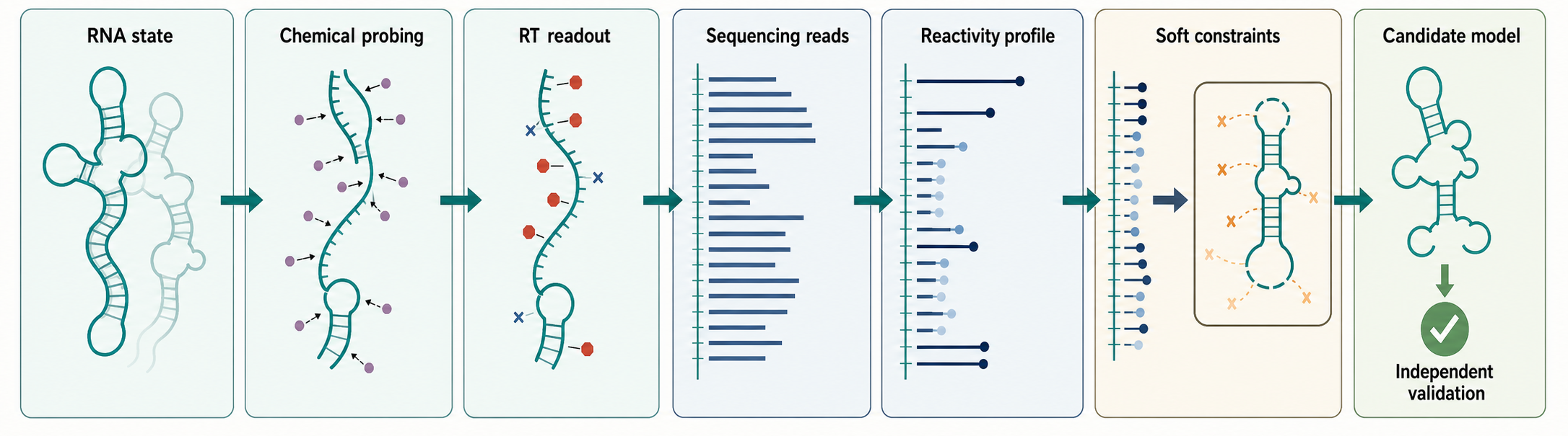
Figure 63.1. Constraint-Data Handoff to Structural Inference. Show Chapter 131 exporting a versioned object containing sequence and coordinate identity, normalized values or pairwise constraints, uncertainty, missingness and coverage masks, condition and replicate metadata, normalization provenance, quality flags, and assay caveats. The inference side transforms this object into soft constraints, priors, likelihoods, candidate contact windows, secondary structures, ensembles, and uncertainty-qualified outputs.
Table 63.1. Constraint-Data Object Fields and Inference Semantics. A structure-constraint record is reusable only when reagent, position, background, normalization, uncertainty, and experimental condition are explicit; otherwise an assay signal becomes an ambiguous pseudo-constraint.
| Field | Required content | Inference use | Failure if absent |
|---|---|---|---|
| Sequence and coordinates | Exact sequence, molecule/isoform, coordinate convention, version | Align values and candidate pairs to modeled residues | Shifted or wrong-isoform constraints |
| Normalized values | Per-position values and assay/reagent semantics | Soft scores, priors, or likelihoods | Scale or chemistry misinterpretation |
| Interaction constraints | Partner coordinates, score, direction and ambiguity | Contact windows or distance-like restraints | Proximity mistaken for a base pair |
| Uncertainty/confidence | Variance, interval, posterior, or quality measure | Weight or qualify observations | All values treated as equally precise |
| Coverage/missingness mask | Informative, excluded, or unmeasured positions | Prevent missing-as-zero errors | Spurious pairing support |
| Condition and replicate metadata | State, treatment, time, compartment, replicate | Differential and hierarchical inference | Incompatible states collapsed |
| Normalization provenance | Method, parameters, software and version | Check scale compatibility and reproduce transforms | False condition differences |
| Quality flags and caveats | Background, ambiguity, saturation, interference and other warnings | Exclude, down-weight, stratify, or model alternatives | Artifacts become confident constraints |
The inference object must first identify what is being modeled. Sequence identity includes the exact nucleotide sequence, molecule or transcript identifier, strand, construct or isoform version, and any known modifications represented by the model. Coordinate identity states whether positions are genomic, transcript-relative, mature-RNA, viral-genome, or construct coordinates. These fields prevent normalized values from being shifted onto the wrong isoform, allele, mature end, or reference version.
For one-dimensional probing, the central data array contains normalized values indexed to the sequence. Each value is accompanied by uncertainty or confidence information when available. A separate missingness and coverage mask distinguishes a measured low value from no information. The inference code must never silently turn missing data into zero reactivity, because zero can be interpreted as evidence favoring pairing. The object also records the assay or reagent class so the mapping function can respect whether a value represents backbone flexibility, selected-base exposure, or another proxy.
For relational measurements, the object contains pairs or regions with normalized interaction scores, coordinate identities for both partners, uncertainty or confidence fields, and flags describing whether the record is intramolecular, intermolecular, directional, ambiguous, or multiply mapped. A proximity or ligation constraint nominates contact, not necessarily canonical pairing. The model may use it as a candidate partner window, a distance-like restraint, or a prior over interacting states, but the encoding must preserve the difference between captured proximity and a verified base-pair register.
Condition and replicate metadata make comparative inference possible. Every profile or contact set should name the organism, cell or biochemical system, compartment when relevant, treatment, time, replicate, RNA selection, and reference annotation. Replicate identifiers must remain visible rather than being collapsed into a mean without variance. Multi-condition inference should compare matched coordinates and carry forward the uncertainty of each condition instead of treating a differential value as error-free.
Quality flags and caveats are first-class model inputs. Control-derived flags can mark high background, low coverage, mapping ambiguity, reagent saturation, inconsistent replicates, isoform ambiguity, known modification interference, or suspected protein protection. The normalization method and version remain attached to the values because different transformations change the scale interpreted by pseudo-energy or likelihood functions. Chapter 131 owns production, measurement benchmarking, and export validation; this chapter decides whether to exclude, down-weight, stratify, or explicitly model flagged observations.
The handoff object should be immutable or versioned once inference begins. A structural result must record the object version, sequence digest or equivalent identity, included conditions, masks, transformation, parameterization, and software version. This provenance makes sensitivity analysis reproducible and prevents a model from being benchmarked against silently revised measurements.
63.2. Mapping normalized reactivities into secondary-structure models
The simplest way to use probing data is visual inspection. A predicted helix should usually correspond to lower reactivity across its paired positions, while loops and junctions should often show higher reactivity. Visual inspection remains valuable because it catches obvious contradictions: a proposed long helix with uniformly high DMS reactivity at A and C residues, a low-reactivity region that the model leaves entirely unpaired, or a reactivity discontinuity at an isoform boundary. Tools that overlay reactivity on structure diagrams or genome browser tracks help modelers perform this first-pass assessment.
Algorithmic integration is more systematic. In a folding program, each candidate secondary structure receives a score. Without probing data, the score is usually derived from nearest-neighbor thermodynamic parameters and loop penalties. With probing data, the score is adjusted. A common SHAPE-directed strategy assigns a pseudo-free-energy term to each nucleotide when that nucleotide is modeled as paired. Low reactivity can provide a modest pairing bonus, and high reactivity can impose a pairing penalty. The algorithm then searches for the structure with the best combined thermodynamic and data-consistency score.
Box 63.1. What Is a Pseudo-Free-Energy Term?
- It is an empirical score adjustment, not a calorimetric free energy.
- Its mapping parameters, normalized input scale, caps, and affected structural states must be reported.
- Soft mappings can tolerate uncertainty; hard rules require independent justification.
- Sensitivity analysis should show whether important helices persist across a defensible parameter range.
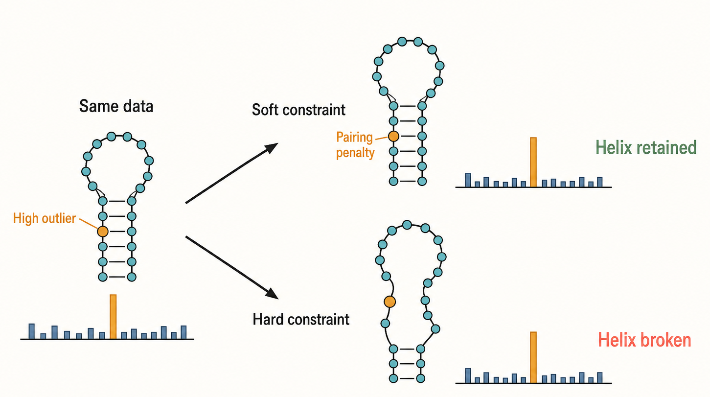
Figure 63.2. Soft Constraints Versus Hard Constraints. Compare a soft score change with a hard required or forbidden state. Use a high-reactivity outlier and a masked nucleotide to show why uncertainty and missingness should change model influence rather than be mistaken for deterministic paired/unpaired labels.
Soft constraints are useful because probing experiments are noisy and RNA molecules are dynamic. If the model used a hard rule that every highly reactive nucleotide must be unpaired, a single chemical outlier could destroy a correct helix. If the model used a hard rule that every unreactive nucleotide must be paired, protein-protected loops and low-coverage positions would be misclassified as helices. A soft constraint lets the folding program violate a reactivity trend when thermodynamic evidence, neighboring data, or comparative evidence strongly favor the violation.
Several inference choices determine the outcome. The first is the transformation from the exported normalized scale to a modeling term. The modeler may cap extreme values for numerical robustness, but must preserve the original object and distinguish an inference transformation from measurement normalization owned by Chapter 131. The second choice is the slope and intercept of the pseudo-energy function. If the pairing penalty is too weak, the data barely matter; if too strong, the algorithm overfits local noise. The third choice is whether the model uses one-dimensional values only, pairwise correlations, multiple conditions, or prior base-pair probabilities. Data-directed probabilistic modeling combines the profile and uncertainty rather than treating values as deterministic instructions.
The distinction between minimum-free-energy structures and ensembles is especially important. A single predicted structure can be helpful for a riboswitch aptamer, a viral untranslated region, or a domain with one dominant fold. For many cellular RNAs, however, base-pair probabilities, alternative structures, and local accessibility may be more honest outputs. A regulatory region may be partly structured in one cell state and remodeled by a protein in another. In that case, the model should report an ensemble shift or a region of changed accessibility rather than claim that the entire RNA has one solved structure.
Chemical modifications add another layer. N(6)-methyladenosine, commonly called m6A, can alter base pairing, stacking, protein recruitment, and chemical readout. A model that includes modified nucleotides may require modified thermodynamic parameters or explicit annotation of modification sites. Methods that predict secondary structure while including m6A show how chemical state can be integrated into folding, but they also illustrate a broader principle: “the sequence” in an RNA folding problem is not always just A, C, G, and U.
63.3. Multi-condition and transcriptome-scale structural inference
Transcriptome-wide probing changes both the scale and the interpretation of RNA structure modeling. In a single-RNA experiment, the modeler often asks whether a particular helix or domain is present. In a transcriptome-wide experiment, the first useful output may be a map of regions that are more or less reactive in vivo than in vitro, during stress than during growth, in one cell type than another, or in one isoform than another. These comparisons can reveal candidate regulatory elements, RNP binding sites, translation-associated remodeling, RNA decay signals, and folding changes linked to disease or viral infection. The output is therefore a structural phenotype, not merely a structure diagram.
Multi-condition inference begins by verifying that the handoff objects are comparable: the same sequence coordinates are aligned, normalized-value semantics match, coverage masks overlap sufficiently, condition labels are correct, and replicate uncertainty is available. Control-derived flags from Chapter 131 remain visible throughout the comparison. Differential reactivity can then identify regions whose accessibility changes. A helix that melts may show increased reactivity across both strands; a protein-protected motif may decrease locally; and a long-range interaction may produce reciprocal changes at distant segments.
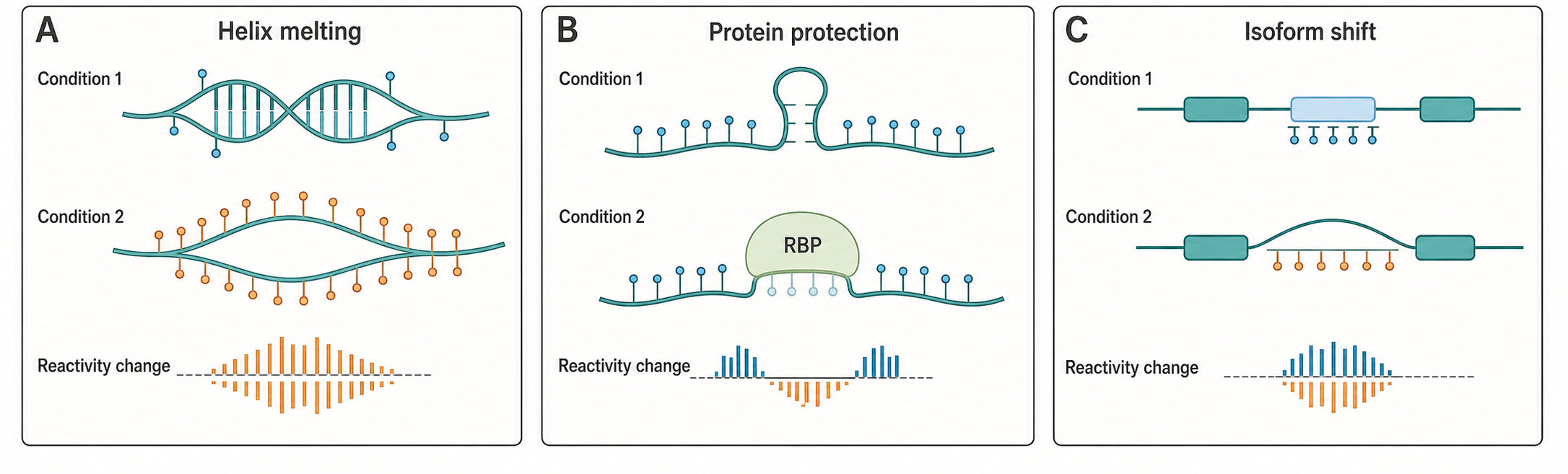
Figure 63.3. Three Explanations for Differential Reactivity. Show helix remodeling, protein protection, and isoform or coordinate mismatch producing superficially similar condition differences. Label the metadata, masks, and additional constraints needed to distinguish them.
The major computational challenge is that transcriptome-wide data are sparse and uneven. Highly expressed RNAs may have excellent coverage, while low-abundance transcripts have missing values. Repetitive regions, paralogous genes, pseudogenes, and overlapping isoforms can produce ambiguous read mapping. Alternative splicing changes which nucleotides are adjacent in the mature RNA. RNA editing and modifications can create apparent mutations in mutational profiling data. For these reasons, transcriptome-wide modeling often focuses on local windows, well-covered regions, or differential signatures rather than full-length structures for every transcript.
Long-read and single-molecule constraint objects address part of the isoform problem by retaining molecule or isoform identity and, when supported, correlations among observations on one molecule. The inference model must still include per-read error or confidence, missing positions, classification uncertainty, and the possibility that an observed molecule does not represent a stable state. Long-read identity reduces coordinate ambiguity but does not by itself solve ensemble assignment.
Single-cell and co-transcriptional probing address two other sources of hidden heterogeneity. Single-cell probing asks whether structural features vary across cells in a population, a question that bulk profiles cannot answer. Co-transcriptional probing asks how nascent RNA folds while RNA polymerase is still synthesizing the transcript. This is important because RNA can form local structures before downstream sequences exist, and those early structures can influence splicing, termination, riboswitch decisions, and RNP assembly. Sequential or time-resolved co-transcriptional probing can capture folding intermediates that are invisible in endpoint measurements.
Multi-condition modeling should not force every change into a secondary-structure explanation. A region can become less reactive because a protein binds, because the RNA enters a granule, because a modification changes reagent chemistry, because a transcript isoform becomes more abundant, or because read coverage changes. The strongest analyses combine probing with orthogonal evidence: RNA-binding protein maps, ribosome profiling, splice isoform quantification, localization assays, structural data, or targeted mutagenesis.
63.4. Integrating RNA-RNA and RNA-protein constraints into structural models
One-dimensional reactivity tells the modeler how each nucleotide behaves, but usually not which partner it contacts. Interaction-constraint objects add relational records: coordinate pairs or regions, normalized scores, confidence, condition and replicate identifiers, ambiguity flags, and assay-specific caveats. Two distant low-reactivity segments can still form separate helices or share protein protection, so relational constraints and one-dimensional values must be integrated without pretending either is a direct base-pair list.
RNA-RNA records nominate candidate intramolecular or intermolecular partners, but the model must decide how to encode them. A high-confidence contact can restrict partner windows, contribute a distance-like penalty, or define an alternative interacting state. Reviews emphasize that contact maps are not automatically base-pair maps. Complementarity, orientation, local reactivity, structural feasibility, replicate support, and ambiguity flags determine whether a precise pairing register is modeled or only a broad proximity restraint.
When RNA-RNA evidence is strong, it can rescue models that one-dimensional probing would leave ambiguous. Consider a bacterial small RNA that represses an mRNA by base-pairing near the ribosome-binding site. DMS probing of the mRNA may show protection near the ribosome-binding site after small RNA expression, but that protection alone cannot tell whether the mRNA forms an intramolecular hairpin, binds a protein, or pairs with the small RNA. A direct RNA-RNA interaction map, combined with compensatory mutations that restore pairing, can support the intermolecular model. The strongest conclusion comes from convergence: changed reactivity at the target site, a captured RNA-RNA contact, sequence complementarity, loss and rescue by mutations, and a functional effect on translation.
RNA-protein constraints have different semantics. A protein-associated region can explain protection, remodeling, or stabilization, but does not prescribe an RNA base pair. Exported binding intervals or scores can annotate regions where low reactivity should not receive an unqualified pairing bonus, define protein-bound states, or stratify condition-specific models. Protein occupancy and base pairing can coexist, so the model should represent compatibility rather than force them to be mutually exclusive.
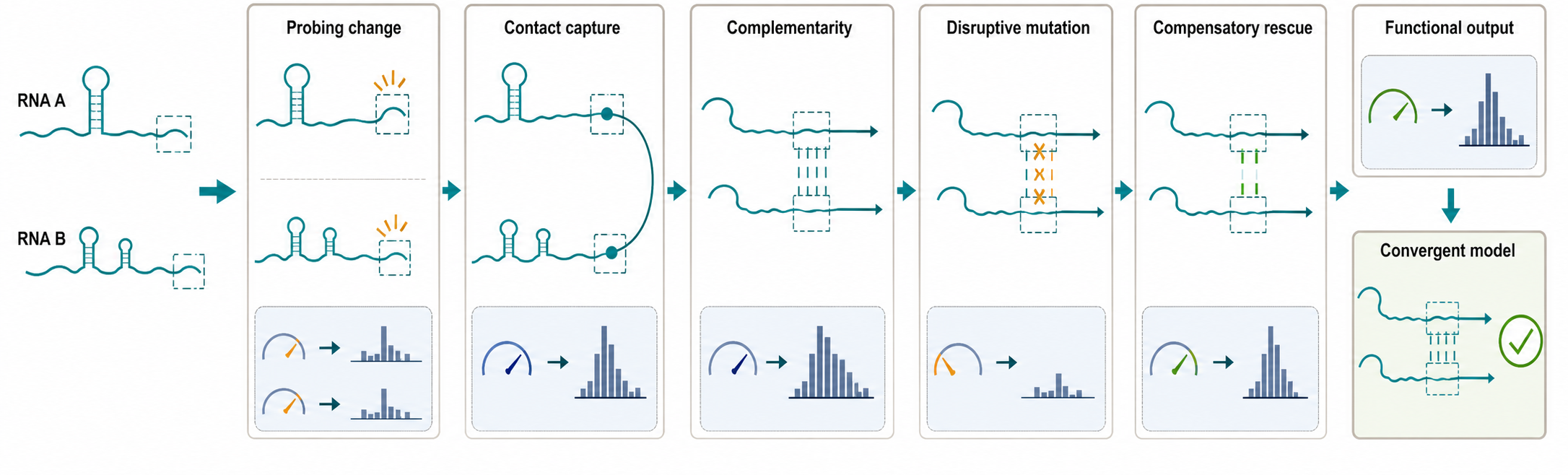
Figure 63.4. Integrating an RNA-RNA Contact. Combine normalized reactivities, a scored pairwise contact, coordinate confidence, complementarity, orientation, comparative support, and disruption/rescue evidence. Distinguish a broad proximity restraint from a verified base-pair register and show how RNA-protein annotations can define alternative RNP states.
Integrative RNP-aware modeling uses protein and RNA-RNA evidence as contextual restraints rather than simple overrides. A protein-binding site may be annotated as “do not interpret low reactivity as base pairing without additional evidence.” An RNA-RNA contact may define candidate pairing windows that are then tested by folding algorithms. A high-confidence RBP motif may explain a local protection pattern. A structural model may include mutually exclusive states: an RNA-only fold, a protein-bound fold, and an intermolecular paired state. This approach fits the biology better than a single diagram pretending that every cell contains one RNA conformation.
63.5. Benchmarking inferred models against structural and comparative evidence
Benchmarking asks whether a probing-constrained model predicts structures that are independently known or strongly supported. The most direct benchmarks use high-resolution structures from X-ray crystallography, nuclear magnetic resonance, or cryo-electron microscopy. A model can be scored by sensitivity, positive predictive value, F1 score, base-pair distance, or agreement with known motifs. These metrics are useful, but they must be interpreted carefully. High-resolution structures often come from stable domains, truncated constructs, engineered RNAs, crystallization conditions, or RNP complexes. A chemical probing experiment may measure a different construct, ligand state, ionic condition, temperature, protein occupancy, or folding pathway. Disagreement can mean the model is wrong, the benchmark is not comparable, or the RNA has multiple states.
Comparative evidence provides another benchmark. If a helix is conserved across homologs through compensatory mutations, the helix has support that is independent of chemical probing. Comparative support is especially valuable for noncoding RNA families, riboswitches, viral structured elements, and conserved untranslated-region elements. A probing-constrained model that recovers covarying helices is more credible than one that contradicts them without explanation. Conversely, probing can help choose among alternative folds when covariation is sparse, when a family has too few sequences, or when a structure is species-specific. Chapter 62 treats comparative methods in detail; this chapter emphasizes that probing and covariation should be cross-checks rather than rivals.
Functional benchmarking is often decisive for regulatory RNAs. If a predicted helix controls translation, splicing, stability, localization, or ligand sensing, mutations that disrupt the helix should alter the function, and compensatory mutations that restore base pairing should restore function. Chemical probing can support the structural interpretation by showing that the disruptive mutation changes the local profile and the compensatory mutation restores it. This strategy is stronger than either functional mutation or probing alone, because it connects sequence, structure, and biological consequence.
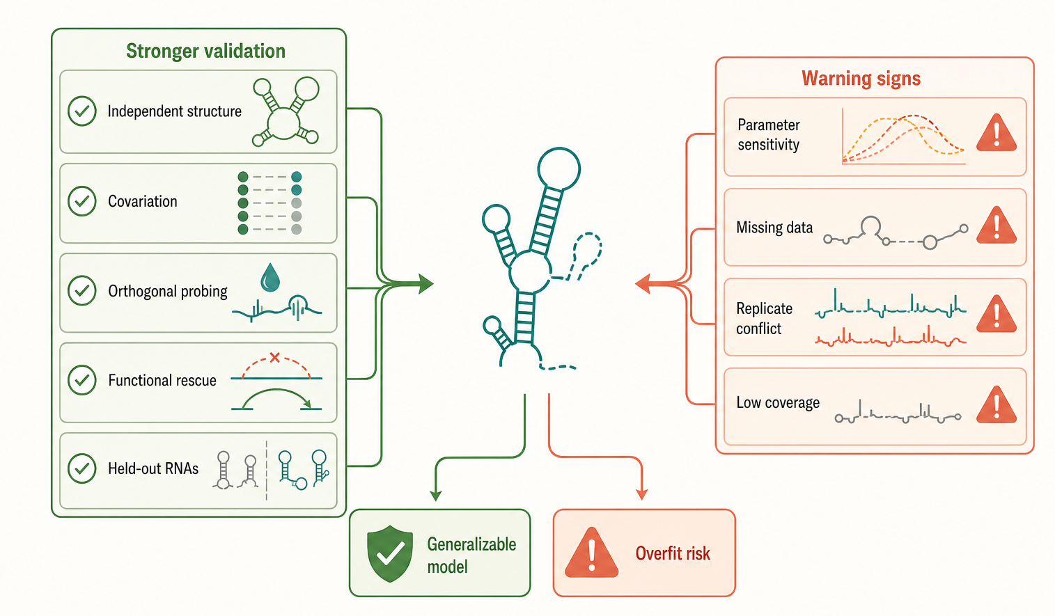
Figure 63.5. Model Benchmarking, Uncertainty, and Overfitting. Separate parameter tuning from held-out evaluation. Compare unconstrained and constrained baselines against state-matched structural or comparative standards; include performance intervals, missing-data stress tests, parameter sensitivity, and warning signs such as benchmark leakage or confident output from sparse constraints.
Computational benchmarking must avoid circularity. If the same RNA families, reagent types, or benchmark structures are used to tune a pseudo-free-energy parameter and then evaluate it, reported accuracy can be inflated. A fair benchmark separates training from testing, includes RNAs of different lengths and architectures, tests multiple reagent types, reports uncertainty, and compares against unconstrained thermodynamic models, comparative models, and simple baselines. It also checks whether the method fails gracefully when given noisy data. A method that returns a confident but wrong structure under weak coverage is more dangerous than a method that reports uncertainty.
The strongest current benchmark evidence combines broad reviews of experimental-data integration with held-out comparisons to independent structural or comparative standards. Accuracy claims should identify the benchmark composition, parameter-tuning split, comparable experimental state, missing-data policy, baseline models, and uncertainty rather than reporting a single pooled score.
63.6. Inference failure modes, uncertainty, and overfitting
Failure Modes and Overfitting to Probing Data
The most common conceptual error is to treat reactivity as base-pair status. High SHAPE reactivity often marks flexible nucleotides, but a flexible nucleotide can occur inside a dynamic helix, at a helix end, in a bulge, in a tertiary contact, or in a protein-remodeled state. Low DMS reactivity at an A or C residue often supports pairing or protection, but it can also reflect protein binding, base modification, poor reagent penetration, low coverage, local sequence effects, or a low-abundance isoform. A reactivity profile is evidence about chemistry under an assay condition. A structure model is an inference from that evidence.
Table 63.2. Inference Failure Modes and Diagnostics. Sparse coverage, mapping error, abundance coupling, incompatible reagents, and overstrong constraints produce different model symptoms; diagnostics should identify the failure before a mitigation or structural conclusion is chosen.
| Failure mode | Model symptom | Diagnostic | Mitigation |
|---|---|---|---|
| Missing treated as zero | Unsupported helices in low-coverage regions | Overlay validity mask | Keep missing values uninformative |
| Overweighted mapping | Fold changes sharply with constraint strength | Parameter sweep | Report stable range and alternatives |
| Incompatible scales | Global condition-specific remodeling | Compare normalization provenance | Harmonize explicitly or avoid pooling |
| Isoform mismatch | Discontinuity near splice boundaries | Verify sequence digest and coordinates | Infer isoforms separately |
| Protein protection as pairing | In-cell-only helix at binding interval | Add protein constraints or depletion state | Model RNP and RNA-only alternatives |
| Contact as base pair | Precise register from broad interaction region | Test complementarity and orientation | Use candidate windows until validated |
| Benchmark leakage | High internal, poor held-out accuracy | Audit train/test families | Use independent state-matched standards |
Overfitting occurs when a model follows noise or assay-specific artifacts so closely that it loses biological plausibility. In secondary-structure prediction, overfitting can happen when pseudo-energy parameters are too strong, when outlier reactivities are not capped, when missing values are treated as zero reactivity, when the same data are used to select and validate a model, or when many alternative models are tried until one looks appealing. Overfitting is especially tempting in large RNAs because there are many possible helices, and a modeler can often find a structure that explains local patches of signal while violating long-range evidence.
Normalization provenance can create or hide structural signals even after handoff. If two objects use incompatible scales, a differential model can confuse transformation with remodeling. The inference layer should not renormalize silently; it should compare the recorded normalization methods, propagate replicate uncertainty, apply coverage masks, and run sensitivity analyses under defensible harmonization choices. Questions about how normalized values and control flags were produced return to Chapter 131.
Protein binding is a major confounder in cells. A protected nucleotide in vivo may be paired, protein-bound, buried in an RNP, chemically modified, or physically inaccessible inside a compartment. Comparing in vitro deproteinized RNA with in vivo RNA can help, but the comparison has its own caveats: deproteinized RNA may refold into a nonphysiological state, lose co-transcriptional history, lose ligands, or change ionic conditions. An RNP-aware interpretation asks which explanation best fits all evidence rather than assuming the in vitro fold is “the RNA structure” and the in vivo profile is a simple perturbation.
Alternative conformations can make a correct biological model look statistically messy. Riboswitches, viral RNAs, repeat-associated RNAs, and many regulatory UTRs can occupy multiple conformations. If two conformations are populated, a bulk reactivity profile may show intermediate values at nucleotides that are paired in one state and unpaired in another. Forcing one minimum-free-energy structure onto such data can produce a hybrid model that no molecule actually adopts. Ensemble modeling, mutate-and-map strategies, single-molecule methods, and condition-specific comparisons are better suited to these cases.
Interaction data have their own failure modes. RNA-RNA ligation can prefer abundant molecules, nearby molecules in condensates, or accessible ends. RNA-protein crosslinking can prefer particular amino acids, nucleotide chemistries, or UV-accessible geometries. A contact between two RNA regions does not prove canonical base pairing. A protein-binding peak does not prove regulation. Integrative modeling improves when every evidence type is assigned the type of statement it can support: proximity, binding, accessibility, pairing, functional effect, or structural geometry.
Table 63.3. Structural Outputs by Inference Question. Minimum-energy structures, ensemble probabilities, constrained comparisons, and model-difference outputs answer different structural questions; the exported object and uncertainty must match the intended inference.
| Question | Appropriate output | Required handoff fields | Overclaim to avoid |
|---|---|---|---|
| Compact RNA with one dominant state | Secondary structure plus confidence | Complete profile, uncertainty, masks | Calling it experimentally solved |
| Dynamic domain | Pair probabilities or state mixture | Condition metadata and uncertainty | Hybrid single fold representing no molecule |
| Transcriptome comparison | Local differential structural phenotype | Matched coordinates, coverage, replicates | Full-length fold for every transcript |
| Isoform-specific structure | Isoform-conditioned profile or ensemble | Molecule/isoform identity and per-read confidence | Treating long-read identity as error-free state assignment |
| Long-range RNA contact | Partner windows and candidate registers | Pairwise scores, ambiguity and orientation | Equating proximity with canonical pairing |
| Protein-bound RNA | RNP-aware alternative states | Protein intervals, condition and caveats | Treating protection as RNA-only helix |
A Practical Modeling Workflow
A defensible inference workflow begins with the output required by the biological question: one secondary structure, an ensemble, local base-pair probabilities, differential accessibility, isoform-specific states, interacting partners, or an RNP-aware model. The output determines which fields of the constraint-data object are informative and which modeling assumptions must be tested.
The second step is handoff-object validation. The modeler verifies the sequence digest and coordinates, object version, normalized scale, uncertainty fields, missingness and coverage masks, condition and replicate labels, quality flags, and assay caveats. Poor-quality or mismatched inputs are not rescued by sophisticated folding software. Visualization tools expose coverage holes, flagged regions, and inconsistent replicates before the modeler becomes attached to a structure.
The third step is model generation with explicit assumptions. The modeler chooses whether to predict one structure, an ensemble, local windows, interacting pairs, or condition-specific states. The modeler records the constraint type, pseudo-energy parameters, normalization, sequence isoform, modification annotations, and any hard constraints. Sensitivity analysis is essential: if a key helix appears only under one arbitrary parameter choice, the helix should not be presented as established. If a helix persists across reasonable parameters and agrees with comparative or functional evidence, confidence increases.
The fourth step is independent validation. Important structural features should be tested by a method that is not merely another transformation of the same reactivity profile. Validation may include compensatory mutations, ligand-dependent rescue, orthogonal probing chemistry, RNase protection, comparative covariation, protein-depletion experiments, CLIP overlap, direct RNA-RNA interaction assays, or high-resolution structural biology. The appropriate validation depends on the claim. A claim that a nucleotide is flexible requires less evidence than a claim that a long-range helix controls splicing in disease.
The final step is uncertainty reporting. A useful model states which helices are strongly supported, which are tentative, which regions are unresolved, and which alternative explanations remain. This is not an admission of failure. It is an accurate representation of what probing-constrained modeling can and cannot infer.
Experimental Foundations and Evidence
The strongest evidence for probing-constrained modeling comes from convergence across chemistry, computation, and independent structure or function. SHAPE-directed modeling showed that experimentally measured reactivity can improve secondary-structure prediction and can be extended to difficult cases such as pseudoknot-containing RNAs when the computational framework allows those features. Probabilistic approaches showed that data-directed folding can represent uncertainty rather than returning only one deterministic structure. Reviews of experimental RNA structure determination and computational modeling summarize the broader consensus that probing data are most valuable when they are integrated with other sources rather than interpreted alone.
High-throughput and transcriptome-wide probing studies extended the evidence base from purified model RNAs to cellular systems. Reviews of RNA structurome methods describe how in-cell and transcriptome-scale probing revealed widespread structure and condition-dependent accessibility, while also emphasizing that cellular reactivity reflects RNP context and assay bias. Nano-DMS-MaP provides an important example of method development driven by biological limitations: short-read probing often cannot distinguish isoforms, while long-read readout can connect structure signals to isoform identity. Long-read single-molecule sequencing further suggests that correlated structural information can be measured along individual molecules, although interpretation still depends on error models and validation.
Interaction-mapping methods broaden the evidence from one-dimensional accessibility to relational constraints. RNA-RNA interaction reviews and primary methods describe how proximity and ligation strategies identify candidate contacts across transcriptomes. RNA-protein interaction reviews describe how CLIP-family and related methods locate binding regions that can explain protection, remodeling, or recruitment. The evidence foundation is therefore not a single method but a layered logic: chemical probing reports nucleotide behavior, thermodynamic models propose base-pairing patterns, interaction maps propose contacts or binding contexts, comparative evidence tests evolutionary conservation, and functional assays test biological consequence.
The evidence is not uniformly mature across all use cases. Targeted SHAPE- or DMS-guided modeling of compact RNAs has a stronger validation base than full-transcript models for low-abundance RNAs in heterogeneous tissues. Single-cell, co-transcriptional, and long-read approaches are rapidly developing and provide crucial new information, but their quantitative modeling frameworks and benchmark standards remain less settled than classic targeted probing. For this reason, this chapter treats some applications as established, others as likely but context-dependent, and others as promising but still benchmark-limited.
Biological Contexts Across RNA Systems
Riboswitches are a natural example for probing-constrained modeling because many riboswitches change structure in response to a small molecule. A ligand can stabilize an aptamer fold, which then changes an expression platform controlling transcription termination or translation initiation. Chemical probing can reveal ligand-dependent protection in the aptamer and structural remodeling in the expression platform. A folding model can propose the helices that connect ligand binding to gene regulation. Functional validation then tests whether mutations disrupt and restore the regulatory switch. This sequence of evidence is a model for causal RNA structure biology.
Box 63.2. Before Trusting a Constraint-Guided Model
- Verify object version, exact sequence, coordinates, condition, and replicate labels.
- Inspect uncertainty, coverage/missingness masks, quality flags, and assay caveats.
- Record the transformation from normalized values to model terms.
- Compare alternative outputs and parameter settings.
- Benchmark against evidence not used to tune or select the model.
- Report unresolved regions and competing structural explanations.
Viral RNAs are another important context. Viral genomes and subgenomic RNAs often contain structured untranslated regions, frameshift elements, packaging signals, replication elements, and long-range interactions. Probing can identify structured regions and condition-dependent remodeling during infection, while RNA-RNA interaction methods can nominate long-range contacts. The difficulty is that viral RNAs are packaged, replicated, translated, and bound by host and viral proteins. A structure measured in virions, infected cells, purified RNA, or replicase complexes may not be the same state. Probing-constrained models of viral RNA should therefore state the experimental state precisely.
mRNAs illustrate why local accessibility can be more useful than full-length folding. A coding transcript may be thousands of nucleotides long, partially covered by ribosomes, bound by RNA-binding proteins, spliced into isoforms, modified, localized, and degraded while being translated. A full minimum-free-energy fold for the entire mRNA is often biologically implausible. More useful outputs include local structure around start codons, upstream open reading frames, splice sites, microRNA target sites, RNA-binding protein motifs, decay elements, and localization signals. Differential probing can identify candidate regulatory regions, but functional interpretation requires translation, splicing, decay, or localization assays.
Long noncoding RNAs raise the isoform and RNP problems sharply. Many lncRNAs are long, low-abundance, nuclear, repetitive, and protein-associated. A reactivity profile may mix isoforms or cell states, and protein protection may dominate RNA-intrinsic folding. Reviews of lncRNA structure and interactome approaches emphasize the need to combine probing, interactome mapping, isoform resolution, and functional perturbation rather than relying on a single predicted fold. Long-read probing and RNA-protein maps are therefore particularly relevant for lncRNA modeling.
Therapeutic and engineered RNAs provide a practical context. Synthetic mRNAs, guide RNAs, siRNAs, aptamers, ribozymes, and RNA devices must fold sufficiently well to perform a designed function, avoid unwanted structures, or maintain manufacturability. Probing can test whether a designed RNA adopts the intended local structure under formulation or cellular conditions. Modified nucleotides and delivery vehicles complicate interpretation because chemical modifications can affect both folding and probing chemistry, and encapsulated or protein-bound RNA may be inaccessible to reagents. Integrative modeling helps distinguish a design failure from an assay-accessibility problem.
Box 63.3. Constraint, Restraint, Evidence, and Measurement
- The measurement is produced and validated in Chapter 131.
- The exported constraint-data object preserves the measurement semantics and caveats.
- A constraint or restraint is one encoding of that evidence in a model.
- Different encodings of the same data can produce different structures.
- A structural model is an inference, not the original observation.
All five figure IDs, three table IDs, and three box IDs continue under registry revision 18. No visual ID is retired in this synchronization.
Technology, Computational, and Clinical Links
Probing-constrained modeling is now part of a broader computational ecosystem. Visualization tools such as IGV-compatible RNA structure tracks, RNAvigate, and web-based structure-data viewers help researchers compare reactivity, structure diagrams, sequencing coverage, and interaction evidence. These tools matter because human error in interpretation often begins before formal modeling: a missing-control region, a low-coverage exon, or a replicate outlier can be overlooked when data are summarized too early.
Machine learning can use probing data in several ways. A model can learn mappings from sequence and probing profiles to base-pair probabilities, classify structured regions, predict reactivity, or prioritize candidate functional elements. Deep learning reviews describe growing interest in RNA structure applications, but they also highlight familiar issues: training data imbalance, benchmark leakage, limited structural ground truth, and difficulty extrapolating to new RNA classes. Probing data can improve learning only when the labels and controls are reliable. A neural network trained on noisy reactivity profiles may learn reagent bias, coverage bias, or transcript abundance rather than RNA structure.
Clinical and translational applications are indirect but important. Disease-associated repeat expansions can form unusual RNA structures and RNP assemblies; probing can help characterize these states, but repeat mapping and cellular heterogeneity are difficult. RNA therapeutics and vaccines require control over sequence, modifications, structure, translation, stability, innate immune recognition, and formulation. Probing can help compare candidate RNA designs or quality-control structural states, but clinical claims require pharmacological, immunological, manufacturing, and safety evidence beyond structure. Structure modeling is one layer in a translational evidence chain, not a substitute for biological testing.
The same principle applies to RNA-targeted small molecules. A compound may stabilize or remodel an RNA structure, and probing can reveal ligand-induced changes. But a reactivity change is not proof of direct binding, selectivity, or therapeutic mechanism. Orthogonal binding assays, mutational mapping, competition experiments, structural biology, and cellular functional assays are needed to establish the mechanism. Probing-constrained modeling is most valuable when it guides these experiments by proposing testable structural hypotheses.
Recent Consensus
The current consensus is that chemical probing has become a central source of evidence for RNA structure modeling, especially when used as a soft constraint and combined with thermodynamic, comparative, interaction, and functional evidence. SHAPE, DMS, icSHAPE, and mutational profiling do not solve RNA structures by themselves. They measure nucleotide behavior under defined chemical and biological conditions. Their greatest strength is that they can be applied to RNAs and states that are difficult for high-resolution structural biology, including large RNAs, cellular RNPs, transcriptomes, isoforms, co-transcriptional intermediates, and changing conditions.
There is also broad consensus that in-cell probing must be interpreted as RNP-aware data. Low reactivity can reflect pairing, protein protection, modification, or inaccessible environment. High reactivity can reflect flexibility, helix breathing, protein-induced remodeling, or exposed loops. Therefore, the best analyses compare conditions, use orthogonal interaction data, report uncertainty, and validate causal claims. A model that is visually pleasing but unsupported by independent evidence is not a final structure.
Computationally, the field has moved from single best structures toward ensembles, differential structure, long-read isoform-aware analysis, single-cell variation, and integrative visualization. Minimum-free-energy diagrams remain useful, but they are no longer the only or always the best output. The relevant output depends on the question: a base-pairing model for a compact ribozyme, base-pair probabilities for a dynamic domain, differential accessibility for a stress response, isoform-specific profiles for alternative splicing, contact maps for long-range RNA-RNA interactions, or an RNP-state model for protein-bound RNAs.
Open Questions, Controversies, Deprecated Models, and Common Misconceptions
Open questions:
- How can researchers model ensembles quantitatively from transcriptome-scale probing data? Bulk profiles often contain mixed states, but many standard pipelines still return one structure or one differential score. Single-molecule, long-read, and single-cell methods are beginning to expose heterogeneity, yet the field still needs stronger statistical models that connect molecular states, readout errors, and biological covariates.
Controversies:
- Another unsettled area is the calibration of probing constraints across reagents, RNA classes, and cellular conditions. A pseudo-free-energy function tuned on one SHAPE reagent and a set of compact RNAs may not transfer cleanly to DMS, icSHAPE, long RNAs, heavily modified RNAs, RNPs, or viral genomes. Multi-reagent integration is conceptually attractive because different chemistries report different features, but the correct weighting is not universal.
- A third controversy is how much transcriptome-wide structure should be interpreted as functional. Structured regions are abundant, and many reactivity changes are reproducible, but reproducibility does not by itself prove biological function. Function requires a causal link to a phenotype, molecular process, or evolutionary constraint. This distinction is especially important for lncRNAs, repeat-associated RNAs, and disease-associated structural hypotheses.
Common misconceptions:
- “Low reactivity means base paired.” Corrected statement: low reactivity means the reagent produced little signal at that nucleotide under that condition. Pairing is one possible explanation, but protein binding, chemical modification, poor coverage, reagent inaccessibility, and ensemble averaging can also produce low signal.
- “A probing-constrained minimum-free-energy structure is experimentally solved.” Corrected statement: a probing-constrained structure is a computational model guided by experimental data. It should be reported with uncertainty, parameter choices, and independent validation for important features.
- “More data always improve the model.” Corrected statement: more data improve a model only if the data are relevant, well controlled, and properly weighted. Combining incompatible conditions, unmodeled isoforms, or biased interaction maps can make a model more confident and less correct.
- “In vitro and in vivo differences are automatically protein effects.” Corrected statement: protein binding is one major explanation, but differences can also arise from ionic conditions, ligand availability, modifications, transcriptional history, RNA concentration, compartment, degradation, or experimental handling.