Chapter 139. Experimental Design, Statistics, Standards, and Reproducibility for RNA Methods
Scope Note
This chapter explains how RNA experiments become interpretable evidence rather than isolated measurements. The focus is not a single assay, but the design logic, statistical reasoning, reporting standards, provenance practices, benchmark construction, and method-selection decisions that determine whether results from RNA extraction, RNA-seq, single-cell RNA-seq, structure probing, RNA modification mapping, CLIP, ribosome profiling, perturbation screens, in vitro selection, and RNA-centric proteomics can be trusted, compared, and reused. The assay-specific mechanics of SELEX and functional-RNA directed evolution belong to Chapter 137; this chapter supplies their general design, uncertainty, provenance, benchmark, and validation framework.
Executive Summary
RNA methods can measure thousands of genes, millions of cells, many nucleotide positions, or many molecular interactions, and this scale makes design failures easy to miss. Confounded batches, insufficient biological replication, weak controls, inappropriate normalization, multiple testing errors, post hoc filtering, and irreproducible workflows can all produce results that look precise but do not support the claimed inference.
The central design unit is the independent biological unit that supports the intended inference: a donor, animal, culture, organoid, infection, plant, microbial colony, treatment vessel, or independently prepared perturbation population, depending on the question. Technical replicates estimate measurement variation but cannot substitute for biological replication. Randomization distributes nuisance variables across conditions; blocking records known nuisance variables so that the design or model can handle them.
Controls and spike-ins make assay outputs interpretable only when they match a specific artifact channel. A positive control shows that the assay can detect a known signal; a negative control estimates background or false-positive behavior; a spike-in monitors steps downstream of its addition point. Batch structure must be designed, recorded, and modeled rather than discovered only after sequencing.
RNA studies routinely test thousands to millions of features, so multiple-testing correction is a basic requirement. Effect size, uncertainty, and power are equally important because adjusted significance alone does not state biological magnitude or precision. Reproducibility also depends on metadata, workflow provenance, FAIR deposition, benchmark scope, negative controls, and method-selection decisions that begin with the biological question rather than with a fashionable platform.
Concept Inventory
- Biological replicate: an independent biological unit that captures variation relevant to the claim.
- Technical replicate: repeated measurement of the same material, library, slide, extract, or reaction.
- Pseudoreplication: treating non-independent observations, such as cells from one donor or tissue spots, as independent biological replicates.
- Randomization: assignment of samples, processing order, lanes, slides, or analysis order to reduce systematic alignment between condition and nuisance variables.
- Blocking: grouping samples by a known nuisance variable, such as donor or batch, while distributing conditions within the group.
- Batch effect: variation caused by processing, reagent, instrument, operator, reference, or pipeline differences rather than by the intended biological contrast.
- Spike-in: an exogenous molecule or cell population added at a defined stage to monitor recovery, scaling, or technical performance.
- Design matrix: a structured representation of experimental variables used by a statistical model.
- False discovery rate: the expected proportion of false positives among called discoveries in a defined family of tests.
- Effect size: the magnitude of a difference or association, such as log2 fold change, binding enrichment, or reactivity change.
- Power: the probability that a study will detect an effect of a specified size under specified assumptions.
- FAIR data: data and digital objects that are findable, accessible, interoperable, and reusable.
- Workflow provenance: the record of software, versions, parameters, references, execution order, and manual decisions that produced a result.
- Benchmark dataset: a dataset designed to evaluate a method against a defined truth source or challenge criterion.
- Gold standard: a reference classification or measurement treated as truth for evaluation, often partial and task-specific in RNA biology.
What to Know Before Reading This Chapter
RNA molecules differ in abundance, length, structure, modification status, subcellular localization, half-life, association with proteins, and extraction efficiency. A method that measures polyadenylated cytoplasmic mRNA is not measuring the full transcriptome; a method that enriches crosslinked protein-RNA complexes is not measuring all binding events; a method that detects modified nucleotides through reverse-transcription signatures is not directly observing chemical groups unless the chemistry and controls support that interpretation.
Most high-throughput RNA experiments convert molecules into counts, intensities, mutation rates, peaks, junction counts, barcodes, spectra, or images. Statistical analysis then compares those measurements across conditions, positions, transcripts, cells, samples, or perturbations. The validity of the comparison depends on whether the experimental units were independent, whether nuisance variables were balanced or modeled, whether controls reveal background processes, and whether the model’s assumptions match the data.
The running examples in this chapter include a bulk RNA-seq treatment comparison, a single-cell RNA-seq atlas, a SHAPE-MaP RNA structure probing experiment, a CLIP experiment for an RNA-binding protein, a ribosome profiling study, and an RT-qPCR validation assay. These examples illustrate a general principle: reproducibility is designed into the study before sequencing or imaging begins, not repaired afterward by a normalization script.
139.1. Replicates, randomization, and experimental design
Experimental design is the plan that links a biological question to a set of measurements capable of answering that question. In RNA biology, the question might be “Which transcripts change after interferon stimulation in primary macrophages?”, “Which RNA regions are bound by an RNA-binding protein?”, “Which ribosome-protected fragments reveal translation of upstream open reading frames?”, or “Which nucleotides become more reactive after ligand binding to a riboswitch?” Each question requires a different measurement, but every question requires a clear definition of the experimental unit, replicate structure, nuisance variables, and planned comparison.
The first decision is the level of biological replication. A biological replicate is not simply another tube, well, lane, or barcode. A biological replicate is an independent biological realization of the condition being studied. If a study asks whether a disease is associated with altered splicing in human skeletal muscle, different patients and control individuals are the biological units. Multiple biopsies from the same patient may be valuable, but those biopsies do not replace independent individuals for population-level inference. If a study asks whether a drug changes mRNA abundance in a clonal cell line under tightly controlled culture conditions, independently seeded, treated, harvested, and extracted cultures can be biological replicates. If a study asks whether a CRISPR perturbation changes gene expression in a pooled screen, the replicate may be an independently transduced and selected cell population, while cells within that population provide many observations but not many independent perturbation experiments.
Technical replicates answer a narrower question: how variable is the measurement process after the biological material has been chosen? Duplicate RT-qPCR wells, repeated mass-spectrometry injections, resequencing of the same library, and repeated imaging of the same tissue section can reveal pipetting variation, instrument drift, stochastic sampling, or local segmentation error. Technical replication is valuable for troubleshooting and quality control, especially in low-input RNA assays. It does not, however, justify claims about biological reproducibility across donors, animals, cultures, or environmental conditions. A technically precise but biologically unreplicated RNA-seq result can have small within-library noise and still be a fragile observation from a single biological case.
Pseudoreplication is one of the most common design failures in modern RNA methods. Single-cell RNA-seq makes the problem vivid. A dataset with 50,000 cells from one treated donor and 50,000 cells from one control donor has many cells but only one donor per condition. Treating cells as independent biological replicates can make confidence intervals artificially narrow and P values misleadingly small because cells from the same donor share genotype, environment, tissue handling, dissociation stress, library chemistry, and batch history. A better design distributes multiple donors across conditions, records donor-level covariates, and uses models or aggregation strategies that respect donor-level independence. The same logic applies to spatial transcriptomics spots from one tissue, CLIP peaks from one library, guide RNAs within one pooled perturbation replicate, or nucleotide positions within one RNA structure-probing experiment.
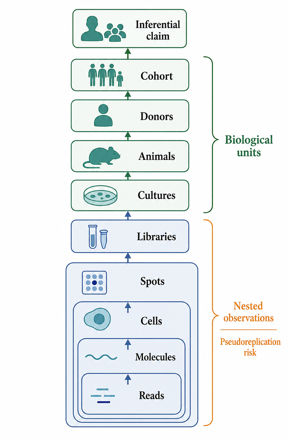
Figure 139.1. Replicate Hierarchy in RNA Experiments. Replication depends on the inferential unit. Reads, cells, peaks, and spots can provide many observations, but biological replication comes from independently generated biological units such as donors, cultures, animals, tissues, or perturbation populations.
Randomization protects the study from systematic alignment between the condition of interest and variables that the investigator did not intend to test. If all control RNA samples are extracted on Monday and all treated samples are extracted on Tuesday, a difference in RNA integrity, reagent lot, operator fatigue, or freezer-thaw interval can masquerade as a treatment effect. If all cases are sequenced on one flow cell and all controls on another, flow-cell effects can become inseparable from biology. Randomization can be applied at treatment assignment, sample processing order, plate position, library index assignment, sequencing lane, imaging order, and data-processing order. Randomization is not merely a formal statistical virtue; it is a practical defense against invisible laboratory gradients.
Blocking is the complementary strategy for known nuisance variables. In a paired design, each donor might contribute a treated and untreated sample, making donor a block. In a time-course infection experiment, each culture batch might include all time points so that batch variation does not align with time. In a spatial transcriptomics study, adjacent sections from the same tissue block might be distributed across stains or capture slides. A block is useful only if it is recorded and included in the analysis or design logic. Blocking without metadata leaves the analyst unable to distinguish intended pairing from accidental clustering.
The design matrix is the computational expression of this logic. For a bulk RNA-seq differential expression analysis, a design matrix might include columns for treatment, donor, batch, sex, RNA integrity number, and a treatment-by-time interaction. For a CLIP experiment, the model might include condition, replicate, immunoprecipitation versus input, crosslinking status, and library depth. For a structure-probing experiment, the comparison might be between reagent-treated and untreated samples, with replicate and transcript abundance as additional factors. The design matrix should be sketched before the experiment begins because some confounding cannot be removed after data collection. If condition and batch are perfectly aligned, no model can determine whether the observed effect belongs to condition or batch.
Table 139.1. Replicate and Design Terms Across RNA Methods. Replicate terminology must be interpreted at the correct experimental level for each RNA method.
| Design term | RNA-method interpretation | Caveat for inference |
|---|---|---|
| Biological replicate | Independent donors, animals, cultures, organoids, infections, plants, microbial colonies, or perturbation populations support biological inference. | Reads, cells, peaks, spots, guides, or nucleotide positions inside one biological unit do not create independent biological replication. |
| Technical replicate | Duplicate RT-qPCR wells, resequenced libraries, repeated imaging fields, repeated injections, or split reactions estimate measurement variation. | Technical precision can reveal assay noise but cannot substitute for independent biological units. |
| Nested observation | Cells within a donor, spots within a tissue section, peaks within a CLIP library, and guide counts within one screen replicate are observations nested inside higher-level units. | Treating nested observations as independent biological replicates creates pseudoreplication unless the model or aggregation strategy respects the hierarchy. |
| Block or paired unit | Donor pairs, culture batches, tissue blocks, time-course batches, plates, or adjacent sections can distribute known nuisance variables across conditions. | Blocking is useful only when block identity is recorded and represented in the design or analysis. |
| Batch | Extraction date, operator, reagent lot, antibody lot, flow cell, capture slide, instrument run, genome build, annotation release, and pipeline version can shift RNA measurements. | Balanced batches can be modeled; condition perfectly aligned with batch cannot be separated reliably after data collection. |
| Primary contrast | Treatment, genotype, time, dose, immunoprecipitation versus input, reagent-treated versus untreated, or guide-target versus control comparisons define the estimable question. | A design matrix cannot recover variables that were omitted, unrecorded, or perfectly collinear with the primary condition. |
The number of replicates should be chosen by expected variability and inferential goal, not by tradition alone. Three biological replicates per condition may detect large, consistent changes in a homogeneous cell-line RNA-seq experiment, but the same number may be inadequate for modest effects in heterogeneous human tissue, single-cell donor studies, isoform-level splicing, RNA modification stoichiometry, or subtle translational efficiency changes. Time-course, dose-response, and factorial experiments require replication across the combinations that support the intended contrasts. A design that includes many conditions with one replicate each is often weaker than a design with fewer conditions and enough replication to estimate variance.
Design also includes preplanned quality criteria. RNA integrity, extraction yield, fragment-size distribution, mapping rate, duplicate rate, fraction of reads in genes, ribosomal RNA contamination, mitochondrial RNA fraction, cell barcode metrics, peak quality, mutation-rate profiles, or library complexity can all reveal failures. Predefined exclusion criteria reduce post hoc bias, but exclusion criteria must be biologically sensible. Removing low-RNA-yield clinical samples may improve technical metrics while systematically excluding necrotic tissue, fibrotic tissue, or vulnerable cell states that are part of the disease biology. Good design therefore records both the technical reason for exclusion and the possible biological implication of exclusion.
A common misconception is that deeper sequencing can compensate for weak experimental design. Sequencing depth reduces sampling noise within a library and can improve detection of low-abundance features, rare junctions, allele-specific transcripts, or small RNA species. Sequencing depth cannot create independent biological replicates, remove perfect confounding, identify an unrecorded reagent lot, or validate an annotation error. Once each library is sufficiently deep for the features of interest, additional libraries from independent biological units often improve inference more than more reads from the same libraries.
Experimental design hands off directly to the method-specific chapters in this part. Chapter 125 expands the design logic for bulk RNA-seq and differential expression. Chapter 126 treats class-specific recovery, modification-aware reverse transcription, and small/stable-RNA normalization. Chapter 127 treats end-chemistry eligibility, coordinate-level end calling, and tail or cleavage controls. Chapter 130 treats donor-level replication, cell-level pseudoreplication, and spatial sampling. Chapter 131 applies replicate and control logic to structure probing. Chapter 133 applies the same principles to CLIP and RNA-protein interaction mapping. Chapter 136 treats pooled perturbation designs, guide-level replication, and screen-level randomization.
Box 139.1. Do Not Overgeneralize Replication
Reads, peaks, spots, and cells are not automatically independent biological replicates. The valid replicate is the independently sampled biological unit that supports the claim, such as a donor, animal, culture, specimen, or perturbation population. Thousands of cells from one donor characterize that donor but do not create thousands of donors; spatial spots are nested within specimens; peaks and reads are nested within libraries. Report both the observation count and the independent-unit count, and use a model that represents the nesting.
139.2. Controls, spike-ins, and batch structure
Controls are observations that make the meaning of assay output more constrained. A positive control asks whether the method can detect a signal that should be present. A negative control asks what signal appears when the target process is absent, blocked, irrelevant, or randomly assigned. A process control monitors a specific laboratory or computational step. A normalization control helps compare samples, but only when its assumptions are valid. RNA methods often need several controls because the measured signal passes through extraction, fragmentation, ligation, reverse transcription, amplification, sequencing, alignment, feature assignment, and statistical modeling.
In RT-qPCR, a no-template control detects reagent contamination or primer-dimer signal; a no-reverse-transcriptase control detects genomic DNA amplification; a standard curve or dilution series tests amplification efficiency; reference genes test normalization assumptions. In RNA-seq, controls may include external RNA spike-ins, replicate libraries, species-mixing experiments, known genotype or sex markers, ribosomal RNA depletion metrics, and orthogonal RT-qPCR for selected features. In CLIP, controls may include input RNA, size-matched input, non-crosslinked samples, immunoglobulin controls, knockout or knockdown of the RNA-binding protein, and binding-deficient mutants. In SHAPE-MaP or DMS-MaPseq, controls include untreated RNA, denatured controls, reagent-free controls, and transcripts with known structures. In ribosome profiling, controls include translation inhibitors or runoff conditions, triplet periodicity, expected coding-region enrichment, and comparison with matched RNA-seq. Chapter 123 gives the assay-specific qPCR, dPCR, blot, FISH, and imaging control logic; this chapter owns the reusable design principles.
Spike-ins are useful but often overinterpreted. A spike-in is an exogenous molecule added to a sample at a defined stage. If a synthetic RNA mix is added before extraction, it can report losses during extraction, degradation, and library preparation. If a spike-in is added after extraction, it cannot report extraction efficiency. If a spike-in is added after reverse transcription, it cannot report reverse-transcription bias. In single-cell experiments, synthetic spike-ins added to a lysis buffer may monitor capture and amplification chemistry, but they do not experience cell lysis, subcellular compartmentalization, RNA-protein complexes, or endogenous RNA structure in the same way as cellular RNA. In crosslinking-based methods, naked synthetic RNAs cannot model protein-shielded endogenous RNAs unless the control is designed for that purpose.
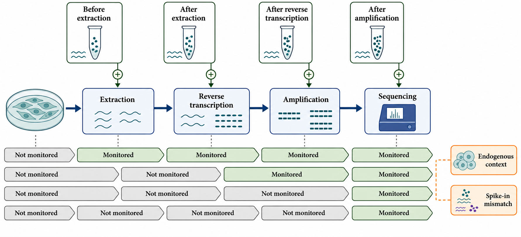
Figure 139.2. What a Spike-In Can and Cannot Monitor. A spike-in reports only the steps downstream of the point where it was added. A spike-in added after extraction cannot measure extraction loss, and a naked synthetic RNA may not mimic endogenous RNA structure, compartment, modification, or RNP association.
Spike-ins also create normalization traps. External RNA controls are sometimes used to infer absolute changes in RNA content per cell. This can be valuable when a treatment globally increases or decreases mRNA abundance, because ordinary library-size normalization can hide global shifts. The inference is valid only if the spike-in amount is proportional to a relevant input unit, such as cell number, tissue mass, or extracted RNA amount, and if the spike-in molecules behave sufficiently like the measured RNAs across samples. If the investigator adds the same spike-in amount to unequal RNA inputs, the spike-in ratio may measure input differences rather than global transcriptional changes. If cell size or total RNA content changes across conditions, the normalization target must be stated explicitly.
Box 139.2. Spike-In Questions Before the Experiment
Before adding a spike-in, define when it enters the workflow, which input unit determines its amount, which losses and biases it experiences, how closely it resembles the endogenous molecules, whether it spans the relevant dynamic range, and which quantity normalization should preserve. A spike-in added after extraction cannot measure extraction loss, and a naked synthetic RNA does not reproduce every structural or ribonucleoprotein constraint of cellular RNA. Fixed spike-in amounts added to unequal inputs can encode the input difference instead of correcting it.
Internal controls are not automatically stable. Housekeeping genes used for RT-qPCR normalization can vary with cell type, proliferation, stress, infection, developmental stage, or drug treatment. Ribosomal RNA abundance can change with growth state and extraction protocol. Small nuclear RNAs and small nucleolar RNAs can change under stress or disease. In miRNA studies, commonly used small RNAs may not be stable across tissues or biofluids. A normalization control should be justified for the specific biological system and perturbation, preferably by empirical stability across the study samples.
Batch structure includes every source of technical or operational grouping that might influence measurement. Examples include extraction date, operator, reagent lot, column lot, plate, well position, index set, PCR cycle number, sequencer, flow cell, lane, capture slide, antibody lot, crosslinking energy, tissue dissociation run, cell-loading channel, mass-spectrometry acquisition batch, reference genome, annotation release, aligner version, and peak-calling parameters. Some batch effects are easy to record and hard to see; others are visible only after exploratory analysis. Principal component analysis, sample correlation heat maps, control-feature behavior, and replicate concordance can reveal batch-associated patterns, but exploratory detection is not a substitute for balanced design.
Table 139.2. Control Types and Artifact Channels. Controls are interpretable when each control is tied to a specific artifact channel.
| Control type | Artifact channel addressed | Evidence or caveat |
|---|---|---|
| Positive control | Confirms that the assay can detect a known RNA signal, binding event, reactivity pattern, translation feature, or perturbation effect. | A positive result proves assay capacity for that control, not universal sensitivity across all transcripts, sites, cells, or conditions. |
| Negative or null control | Estimates background signal from nonspecific recovery, random assignment, off-target perturbation, ambient RNA, or false-positive calling. | The negative control must match the artifact channel; one null control rarely covers contamination, binding specificity, and modeling error at once. |
| Process control or spike-in | Monitors recovery, scaling, capture, library preparation, reverse transcription, amplification, or sequencing steps downstream of the addition point. | A spike-in added after extraction cannot measure extraction loss, and naked synthetic RNA may not mimic endogenous RNPs, modifications, or compartments. |
| Input or size-matched input | Helps distinguish enrichment from transcript abundance, accessibility, fragmentation, or library-depth differences in CLIP and related capture assays. | Input controls do not prove direct binding or functional regulation; they define a comparison background. |
| Knockout, knockdown, or binding-deficient control | Tests whether signal depends on the targeted RNA-binding protein, writer enzyme, perturbation reagent, or binding domain. | Loss of signal supports target dependence, but incomplete depletion, compensation, toxicity, and indirect effects still need evaluation. |
| No-template and no-reverse-transcriptase controls | Detect reagent contamination, primer-dimer products, or genomic DNA amplification in RT-qPCR and related assays. | These controls address reaction contamination and DNA carryover, not biological replication or global normalization. |
| Species-mixing, empty-droplet, or hashing controls | Reveal barcode swapping, ambient RNA, doublets, multiplets, and sample mixing in single-cell and spatial workflows. | They estimate specific single-cell artifacts but do not remove donor-level confounding or validate cell-type interpretation. |
| Orthogonal validation | Tests whether a discovery survives a different measurement principle, such as RT-qPCR, digital PCR, imaging, mass spectrometry, mutagenesis, or biochemical binding. | Validation is strongest when it samples positives, borderline calls, and negative controls rather than only the most favorable discoveries. |
Batch correction is a modeling operation, not a magic eraser. When batches are balanced across conditions, models can estimate and adjust for batch-associated variation while preserving biological contrasts. When batches are nested within conditions, batch correction may remove real biology, preserve technical artifacts, or create artificial structure. In single-cell integration, aggressive batch correction can align biologically distinct cell states if the method assumes shared populations across datasets. In spatial transcriptomics, correction can remove tissue-region signals if those regions are confounded with slides. In CLIP, peak differences can reflect antibody lot or crosslinking efficiency; a correction that ignores immunoprecipitation biology may overstate precision.
Controls must match the claim. A negative control for nonspecific antibody binding does not prove that a CLIP peak is functionally regulatory. A spike-in control for extraction efficiency does not prove that an RNA modification call is chemically correct. A no-reverse-transcriptase control does not validate a differential expression model. An empty-droplet control in single-cell RNA-seq does not eliminate doublets. Each control narrows a specific artifact channel. Strong evidence often comes from a ladder of controls: process controls to show the assay worked, negative controls to define background, positive controls to show sensitivity, perturbation controls to test target dependence, and orthogonal methods to confirm biological interpretation.
Boundary cases deserve explicit planning. Clinical samples may arrive in nonrandom order because cases and controls are collected at different clinics. Developmental time-course samples cannot be fully randomized across time, but processing can be blocked and balanced. Rare primary cells may be too limited for all ideal controls; in that case, pilot experiments in accessible systems can characterize technical artifacts, while the precious samples are reserved for the primary contrast. Viral infection studies may require biosafety batching that cannot be randomized completely. The correct response is not to hide these constraints, but to record them, model what can be modeled, and avoid claims that the design cannot support.
The evidence basis for control choice often comes from method-comparison studies, standards documents, and accumulated failure cases. Quantitative PCR reporting standards, high-throughput sequencing reporting standards, single-cell metadata recommendations, and community repository rules have all emerged because missing controls and missing metadata repeatedly made published results difficult to interpret. The chapter-local reference file for this chapter does not yet contain curated anchors for these standards; the reference section therefore lists citation targets requiring expert curation rather than treating memory-based citations as final.
139.3. Multiple testing, effect sizes, power, and uncertainty
RNA methods usually produce many tests. A bulk RNA-seq study may test 15,000 to 25,000 genes. A transcript-level analysis may test more isoforms than genes. A splicing analysis may test exon-inclusion events or junctions. A CLIP study may test binding peaks or motif enrichments. A SHAPE-MaP study may test nucleotide reactivities across many transcripts. A single-cell atlas may test marker genes across many clusters, differential abundance across many cell states, and perturbation effects across many guide RNAs. Without multiple-testing correction, some features will appear significant by chance simply because the study asked many questions.
The false discovery rate, or FDR, is the expected proportion of false discoveries among the set of discoveries called under a defined testing procedure. FDR control is commonly used in RNA studies because investigators often prefer a discovery list with a tolerable expected fraction of false positives over a procedure so conservative that it misses most real signals. The Benjamini-Hochberg procedure is a standard FDR method under independence or certain positive-dependence conditions, and related methods address more complex dependence structures. The important practical point is that the family of tests must be defined. Testing all genes, then reporting only a pathway subset without acknowledging the original test family, changes the interpretation of adjusted values.
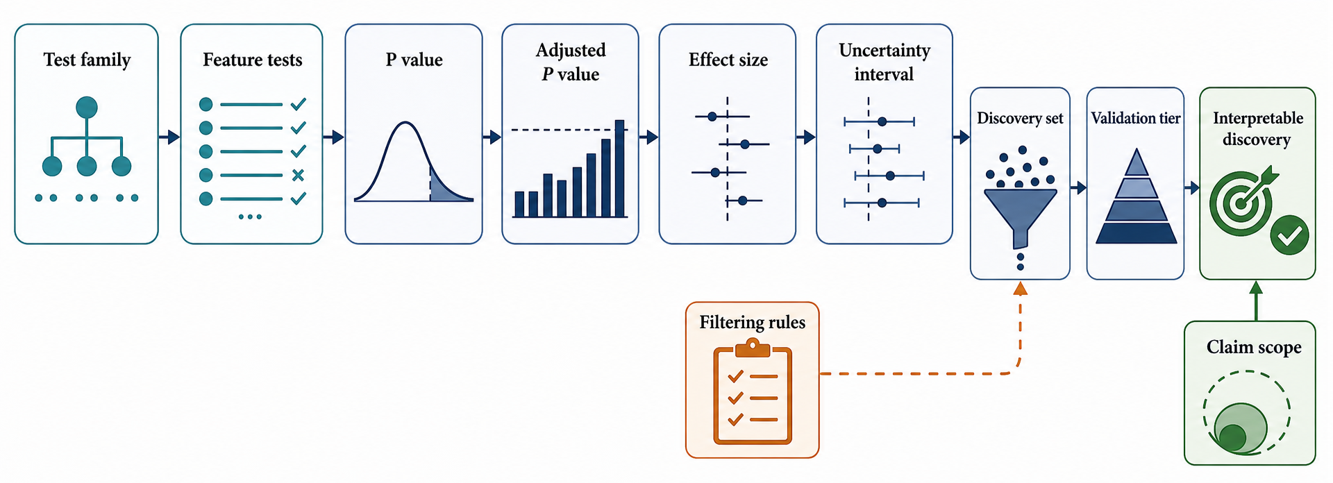
Figure 139.3. From Many Tests to Interpretable Discoveries. Transcriptome-scale discovery requires a defined test family, multiple-testing correction, effect-size interpretation, uncertainty reporting, and validation appropriate to the biological claim.
Adjusted P values do not measure effect magnitude. A tiny fold change can have a very small adjusted P value in a large, precise dataset, while a large biological effect can be statistically uncertain in a small or noisy dataset. RNA chapters often distinguish several effect-size scales: log2 fold change for transcript abundance, percent-spliced-in difference for alternative splicing, change in translational efficiency for ribosome profiling, difference in mutation rate or reactivity for structure probing, peak enrichment for CLIP, modification stoichiometry difference for epitranscriptomic assays, and cell-state proportion difference for single-cell data. An effect size must be interpreted in the context of measurement scale and biological consequence. A twofold change in a rare transcript may be less consequential than a 15 percent change in a dosage-sensitive regulatory RNA, and a small change in a ribosomal protein mRNA may reflect a coordinated growth program.
Uncertainty describes how precisely a study estimated an effect. Confidence intervals, credible intervals, standard errors, bootstrap intervals, posterior distributions, and replicate concordance metrics all serve this purpose in different frameworks. A result reported as “log2 fold change 1.2, FDR 0.01” is less informative than a result that also reports the interval, baseline abundance, replicate variability, model design, and whether the effect was observed across biological replicates. In RNA modification mapping, uncertainty may include site-level detection confidence and stoichiometry error. In single-cell annotation, uncertainty may include classifier probabilities, marker ambiguity, and donor-level variability. In structure probing, uncertainty includes read coverage, mutation-rate background, and model dependence when reactivities are converted into structures.
Power is the probability of detecting an effect of a given size under the planned design. It is not a property of a method in isolation. Power depends on biological variance, technical variance, number of independent replicates, sequencing depth, feature abundance, dispersion, dropout, cell composition, batch structure, and the statistical model. In bulk RNA-seq, additional biological replicates improve estimation of dispersion and donor variability. In single-cell RNA-seq, adding more cells can improve characterization of cell states within a donor, but adding more donors is usually required for population-level condition effects. In CLIP, more reads may improve peak resolution, but independent immunoprecipitations and antibody validation determine whether binding calls reproduce. In ribosome profiling, depth, fragment periodicity, matched RNA-seq, and replicate concordance all affect power to detect translation changes.
Table 139.3. Statistical Quantities and RNA-Specific Examples. Statistical quantities in RNA methods must be tied to measurement scale, model assumptions, and biological interpretation.
| Statistical quantity | RNA-specific example | Interpretation caveat |
|---|---|---|
| Adjusted P value | Gene-level differential expression, CLIP peak tests, splicing-event tests, marker-gene tests, or nucleotide-reactivity tests after multiple-testing correction. | It is not the probability that one specific feature is false, and it does not state the biological magnitude of the effect. |
| False discovery rate | Expected fraction of false positives among called discoveries in a defined gene, transcript, peak, site, guide, or cluster test family. | The test family and filtering rules must be stated; changing the family after looking at the results changes interpretation. |
| Effect size | log2 fold change, percent-spliced-in difference, translational-efficiency change, peak enrichment, reactivity difference, modification stoichiometry, or cell-state proportion shift. | Large datasets can make tiny effects significant, while large biological effects can remain uncertain in noisy or underpowered designs. |
| Confidence or credible interval | Interval around a fold change, enrichment, stoichiometry estimate, cell proportion, or structure-probing reactivity. | Interval meaning depends on the statistical framework and on whether the model captures replicate, batch, and feature-level dependence. |
| Power | Probability of detecting a specified abundance, splicing, binding, translation, modification, or perturbation effect under the planned design. | More reads or cells improve some measurements but do not create independent donors, cultures, immunoprecipitations, or screen populations. |
| Dispersion or variance model | RNA-seq count dispersion, donor variability, guide-level variation, dropout, overdispersion, or replicate-to-replicate peak variability. | Dispersion estimates are fragile with too few biological replicates and can be distorted by hidden batch effects. |
| Calibration | Agreement between reported probabilities, FDRs, confidence scores, or classifier scores and observed error rates in held-out benchmarks. | A well-ranked discovery list can still be poorly calibrated for decision thresholds, clinical use, or mechanistic claims. |
| Feature filtering | Minimum counts, coverage thresholds, peak reproducibility filters, site-quality filters, or cell-quality filters before testing. | Independent filtering can improve power, but outcome-driven filtering can bias significance and hide the true discovery space. |
Power analysis for RNA methods is often approximate because variance structures are complex. Pilot data, public datasets, simulation, downsampling, and method-specific power tools can help estimate required sample sizes. The assumptions should be written down: expected effect size, expected dispersion, planned FDR threshold, minimum abundance filter, sequencing depth, replicate number, donor variability, and primary contrast. A power calculation based on homogeneous cell lines should not be silently transferred to heterogeneous human tissue. A power calculation based on gene-level expression should not be silently applied to isoform-level inference, rare cell-state detection, or nucleotide-resolution modification mapping.
Statistical models should follow the design rather than retrofit the desired conclusion. Count models for RNA-seq commonly account for mean-variance relationships and library-size factors. Linear models, generalized linear models, mixed models, beta-binomial models, hierarchical models, permutation tests, and Bayesian models each fit particular data structures. A paired donor design should be analyzed as paired. A multi-batch design should include batch terms or use a method that addresses batch structure. A screen with multiple guide RNAs per target should account for guide-level behavior and target-level aggregation. A spatial or single-cell dataset should account for dependence among cells, spots, fields, donors, and samples. When the model ignores the experimental unit, the reported uncertainty often becomes too optimistic.
Feature filtering must be principled. Removing features with extremely low counts can improve power by reducing the multiple-testing burden and avoiding tests with little information. Filtering based on the outcome, such as keeping genes that appear different between conditions before formal testing, can bias significance. In CLIP, filtering peaks by reproducibility across replicates is often useful, but the filtering criterion should be independent of the particular contrast being tested or handled in a statistically coherent way. In RNA modification studies, coverage filters and signal thresholds must be reported because they shape which sites can be discovered.
Multiple testing also affects validation. Selecting the top five genes from a genome-wide RNA-seq experiment for RT-qPCR validation does not estimate the false discovery rate of the full list. It tests a biased subset enriched for strong signals. Orthogonal validation is valuable, but it should include positive examples, borderline examples, and negative or unchanged controls when the goal is to evaluate the discovery procedure. Similarly, validating one prominent CLIP peak by reporter assay does not validate all peaks; validating one methylation site by mass spectrometry does not validate all antibody-enriched sites; validating a few cell-type markers does not validate all cluster labels.
Misinterpretations of P values are common enough to merit direct warning. A P value is not the probability that the null hypothesis is true. An adjusted P value is not the probability that a specific gene is a false positive. Failure to reach significance is not proof of no effect, especially in underpowered studies. Statistical significance is not proof of mechanism. In RNA biology, mechanism usually requires additional evidence: perturbation, dose response, temporal order, biochemical reconstitution, direct binding, structural evidence, genetic rescue, or orthogonal measurement.
Recent consensus in high-throughput RNA analysis favors reporting effect sizes and uncertainty alongside adjusted significance; defining test families; using models that match count distributions and design structure; avoiding pseudoreplication; documenting filtering; and validating claims with controls appropriate to the biological conclusion. Open questions remain about best practices for complex multiomic single-cell designs, spatial autocorrelation, isoform-level uncertainty, direct RNA sequencing error models, RNA modification stoichiometry, and benchmark-based calibration of new machine-learning methods.
139.4. Metadata, workflow provenance, and FAIR deposition
Metadata are data about the data: the sample, organism, cell type, tissue, disease state, genotype, sex, age, treatment, time point, collection method, extraction chemistry, library construction, sequencing platform, computational pipeline, and analysis decisions that allow another scientist to interpret the measurements. Metadata are not bureaucratic extras. Without metadata, a count matrix becomes a set of numbers detached from biological meaning. A matrix labeled only “treated” and “control” cannot support serious reuse if the reader cannot determine whether the samples were primary tissue, cultured cells, sorted cells, nuclei, organoids, infected cells, or synthetic constructs.
Minimum metadata for an RNA experiment should identify the biological source, experimental design, sample processing, assay protocol, instrument, raw data, processed data, and analysis workflow. For a human single-cell RNA-seq study, this may include donor identifiers, consent or access restrictions, tissue source, dissociation protocol, viability, enrichment or sorting strategy, chemistry version, cell-loading concentration, sequencing metrics, genome build, annotation release, cell-calling method, doublet detection, ambient RNA correction, clustering method, marker-based annotation, and donor-level covariates. For a bacterial RNA-seq experiment, the critical metadata may include strain, growth medium, temperature, growth phase, stress exposure, RNA stabilization, rRNA depletion, strand specificity, and operon-aware analysis choices.
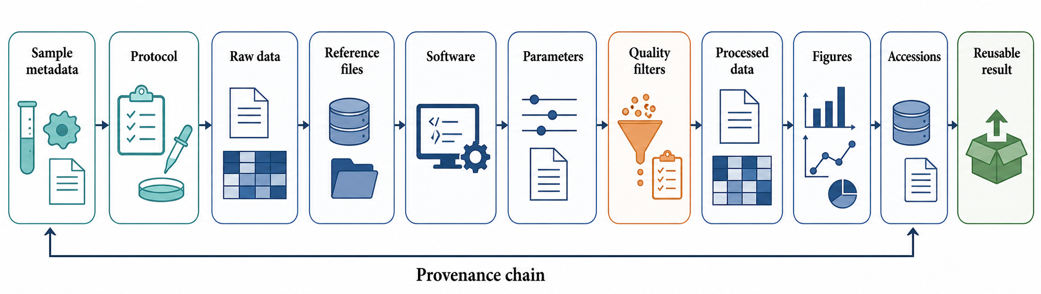
Figure 139.4. Provenance Chain from Sample to Result. Reproducibility requires a continuous provenance chain linking biological source, protocol, raw observations, computational references, software versions, parameters, filtering decisions, and final results.
Workflow provenance records how raw observations became results. A modern RNA result often passes through base calling, demultiplexing, adapter trimming, quality filtering, alignment or pseudoalignment, duplicate handling, feature assignment, normalization, statistical modeling, visualization, and manual interpretation. Each step has software versions, reference files, parameters, and thresholds. Reference genome and annotation versions are especially important because transcript models, gene symbols, pseudogene annotations, repeat annotations, small RNA loci, and splice junctions change over time. A differential expression result based on one annotation release may not be identical under another.
Reproducible computational workflows use scripts or workflow managers rather than undocumented point-and-click histories. Containers, environment lock files, notebooks with fixed inputs, checksums, and version-controlled code can reduce ambiguity. Random seeds should be recorded when stochastic algorithms affect cell clustering, dimensionality reduction, subsampling, simulation, or model initialization. Manual curation should be described as a decision procedure, not hidden as “data cleaning.” For example, if cell clusters were merged because marker genes and transcriptome similarity supported a shared identity, the markers and criteria should be recorded.
FAIR data principles summarize a broad target: data should be findable, accessible, interoperable, and reusable. Findability requires persistent identifiers, searchable metadata, and repository registration. Accessibility requires clear access routes, authentication conditions when needed, and long-term availability. Interoperability requires standard formats, controlled vocabularies, ontologies, and machine-readable links where possible. Reusability requires enough metadata, provenance, license or access information, and quality context for others to determine whether the data fit a new purpose. FAIR does not necessarily mean unrestricted public access; controlled-access human genomic data can be FAIR when metadata, access procedures, and reuse conditions are clear.
Deposition should include raw data whenever lawful and practical. Raw reads, raw signal files, raw images, or raw spectra allow reanalysis when aligners, references, annotations, or algorithms improve. Processed data are also necessary because many users cannot reconstruct a study from raw files alone. A useful RNA deposition often includes raw sequence files, processed count matrices or peak files, sample metadata, protocol details, code, workflow descriptions, quality-control metrics, and final analysis tables. For single-cell data, cell-level metadata and embeddings may be useful, but they do not replace raw reads and donor-level metadata. For spatial data, images, spot coordinates, tissue annotations, and processing outputs must remain linked.
Table 139.4. Minimum Metadata for Reusable RNA Datasets. Reusable RNA datasets require sample, protocol, instrument, reference, software, quality-control, and access metadata.
| Dataset class | Minimum reusable metadata | Reuse caveat |
|---|---|---|
| Bulk or targeted RNA-seq | Biological source, strain or donor covariates, treatment, time point, RNA integrity, extraction chemistry, depletion or selection strategy, strandedness, library kit, sequencer, depth, genome build, annotation release, count method, and design matrix. | A count table without sample, protocol, and reference metadata cannot support reliable reanalysis or comparison. |
| Single-cell or single-nucleus RNA-seq | Donor and sample identifiers, tissue handling, dissociation or nuclei isolation, viability, enrichment strategy, chemistry version, loading concentration, barcode metrics, cell-calling, doublet handling, ambient RNA handling, clustering, annotation criteria, and donor-level covariates. | Cell-level metadata do not replace donor-level metadata for population inference. |
| Spatial transcriptomics | Tissue source, fixation or freezing, section thickness, capture chemistry, imaging, spot or cell coordinates, registration, tissue annotations, segmentation, resolution, sequencing metrics, and linked histology files. | Spatial reuse fails when images, coordinates, regions, and expression matrices are deposited separately or without shared identifiers. |
| CLIP, RIP, or RNA-protein interaction mapping | Crosslinking condition, antibody or tag, input control, knockout or depletion control, nuclease digestion, ligation steps, size selection, replicate identity, peak caller, genome build, annotation, and background model. | Peak files alone do not distinguish direct contact, nonspecific recovery, abundance effects, or functional regulation. |
| RNA structure probing | Probe reagent, in vitro or in-cell context, untreated and denatured controls, reaction time, temperature, transcript abundance, mutation-rate background, coverage filters, normalization, and folding constraints. | Reactivity is an assay output, not structure itself; downstream models and control choices must be recorded. |
| RNA modification mapping | Target mark, enrichment or chemistry, antibody or enzyme information, standards, knockout or perturbation controls, direct-RNA signal model when relevant, site-calling thresholds, stoichiometry assumptions, and validation method. | Region or site calls are hard to reuse without specificity controls and explicit thresholds. |
| Ribosome profiling | Harvest conditions, inhibitor or runoff strategy, nuclease digestion, protected-fragment size range, periodicity metrics, matched RNA-seq, coding-region enrichment, start-site handling, and translational-efficiency model. | Ribosome footprints indicate ribosome occupancy and require matched evidence before being treated as completed protein output. |
| Pooled perturbation screens | Library design, guide or reagent sequences, target mapping, multiplicity, coverage, selection conditions, replicate populations, barcode assignment, non-targeting and positive controls, sequencing depth, and target-level aggregation method. | Guide counts are nested within perturbation populations; off-target effects and bottlenecks must be visible in the metadata. |
| Cross-cutting workflow provenance | Raw-data accessions, checksums, software names and versions, containers or environment locks, reference files, parameters, random seeds, quality thresholds, manual curation rules, processed outputs, and license or access terms. | FAIR deposition can be controlled-access, but users still need identifiers, metadata, access procedures, and reuse conditions. |
Standard formats make reuse more likely: FASTQ for reads, BAM or CRAM for alignments, BED-like files for intervals, GTF or GFF for annotations, matrix formats for counts, HDF5-based containers for many single-cell objects, and specialized formats for spectra, images, and spatial coordinates. Format choice is only one layer. Identifiers, coordinate conventions, genome build, strandedness, barcode definitions, and feature naming must also be documented.
Reporting standards and checklists help authors remember what to report. Quantitative PCR has minimum-information guidelines; sequencing experiments have minimum-information expectations; single-cell studies have metadata recommendations; proteomics and imaging communities have their own reporting standards. These standards are not substitutes for scientific judgment. A checklist can ensure that primer sequences, amplification efficiencies, genome builds, and software versions are reported, but it cannot decide whether the design answered the biological question. Conversely, a well-designed study can become difficult to reuse if it ignores reporting standards.
Privacy, ethics, and consent shape deposition for human RNA data because transcriptomes and clinical metadata can reveal sensitive participant information. Reproducibility therefore requires controlled-access repositories, deidentified metadata, consent-compatible use terms, and explicit access restrictions.
Boundary cases include proprietary clinical assays, public-health outbreak data, endangered species samples, indigenous data governance, and dual-use pathogen studies. FAIR deposition may then require metadata records, summary data, controlled workflows, synthetic examples, or delayed release rather than full open release.
The evidence basis for metadata and provenance standards comes from the repeated observation that missing sample annotations, missing raw data, missing code, and ambiguous genome builds prevent reuse. Method chapters in this book treat the assay-specific details. Chapter 144 expands repositories, workflow managers, ontologies, and FAIR systems. This chapter provides the design-level bridge: the study must plan metadata capture before the experiment begins, because many metadata fields cannot be recovered later.
139.5. Benchmark datasets, gold standards, and negative controls
A benchmark dataset is a deliberately chosen dataset used to evaluate a method. A gold standard is the set of labels, measurements, or truth assignments against which the method is judged. A negative control is a sample, feature set, perturbation, or comparison expected not to contain the target signal. These concepts are related but not interchangeable. A benchmark without a credible reference standard may measure convenience rather than accuracy. A gold standard without negative controls may conceal false-positive behavior. A negative control without a realistic data-generating process may underestimate artifacts in real experiments.
Benchmarks are necessary because RNA methods often optimize one property while sacrificing another. An aligner may be fast but weak for repetitive transcripts. An isoform quantifier may perform well for abundant transcripts but poorly for paralogous genes. A single-cell integration method may remove batch effects but blur real cell-state differences. A CLIP peak caller may be sensitive but call many background peaks. A structure prediction method may fit canonical base-paired RNAs but fail on pseudoknots, ligand-dependent switches, or protein-stabilized folds. A benchmark makes these tradeoffs visible if the benchmark includes realistic variation and appropriate metrics.
Gold standards in RNA biology are often imperfect. In differential expression, known mixtures of RNA samples can define expected fold changes for some genes, but mixture designs may not capture biological regulation, RNA processing, or cell-state shifts. In isoform analysis, synthetic spike-ins and simulated reads can define transcript abundance, but simulations may not capture reverse-transcription bias, fragmentation bias, or ambiguous mapping in real genomes. In RNA modification detection, mass spectrometry can validate global chemical composition but may lose site information; antibody enrichment can locate regions but may have specificity problems; direct RNA sequencing can preserve native RNA but has error-model challenges. In CLIP, binding sites confirmed by biochemical assays or genetic perturbation are valuable, but known sites are biased toward well-studied proteins and abundant transcripts.
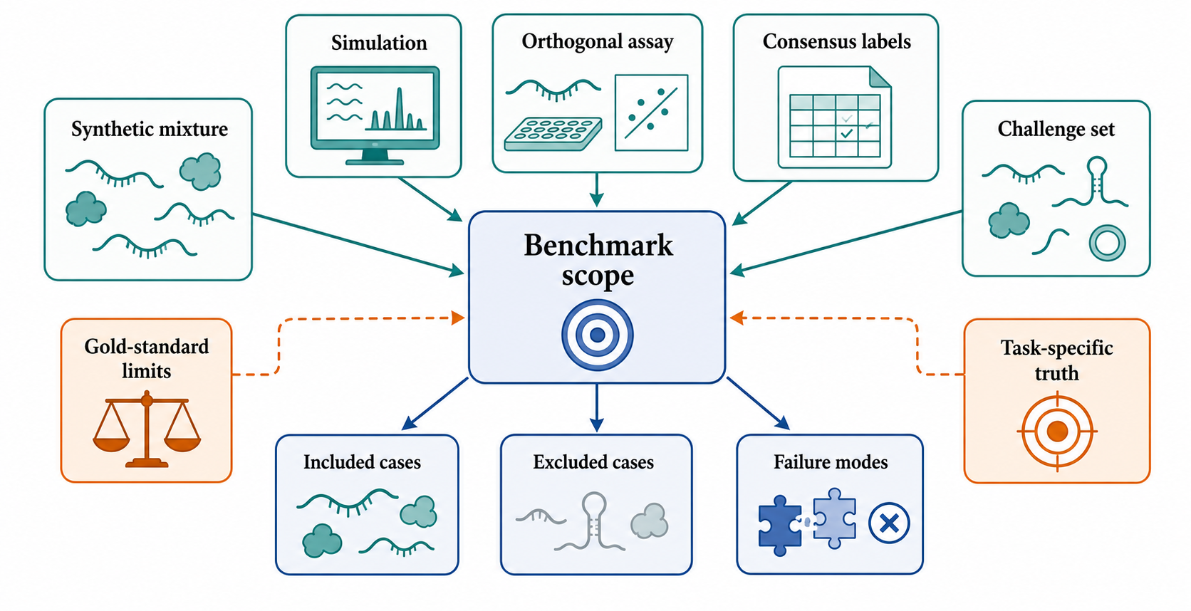
Figure 139.5. Benchmark Scope and Gold-Standard Limits. Gold standards for RNA methods are usually partial and task-specific. A benchmark must state what truth source it uses, which cases it excludes, and which method failures it can reveal.
A good benchmark specifies the task. “Best RNA-seq method” is not a meaningful benchmark target. The target might be gene-level differential expression in bulk samples, isoform quantification in a mammalian genome, rare-cell detection in single-cell data, allele-specific expression, fusion detection, editing-site detection, m6A peak detection, ribosome occupancy, protein-RNA binding site localization, or RNA structure reactivity estimation. Each task needs different truth labels and metrics. Sensitivity, specificity, precision, recall, FDR, calibration, root-mean-square error, rank correlation, reproducibility, runtime, memory use, and robustness to degraded RNA may all matter, but not equally.
Negative controls reveal how methods fail. In CLIP, a nonbinding protein, knockout sample, or non-crosslinked sample can expose nonspecific recovery and background peaks. In RNA modification mapping, unmodified synthetic RNA, enzyme knockout, chemical demethylation, or orthogonal chemistry can test false modification calls. In single-cell RNA-seq, empty droplets, species-mixing experiments, and cell hashing controls can reveal ambient RNA, barcode swapping, and doublets. In perturbation screens, non-targeting guides, safe-targeting controls, and positive-control guides define null and expected-effect distributions. In spatial transcriptomics, blank capture spots, tissue-free regions, and known anatomical markers reveal background and misregistration.
Negative evidence is not failure; it is information about boundaries. If a claimed lncRNA knockdown produces no reproducible phenotype across independent reagents, the result constrains mechanism. If an RNA-binding protein shows many CLIP peaks but depletion does not alter target RNA abundance, the finding may indicate binding without regulation, regulation of translation or localization rather than abundance, compensation, or false-positive binding. If a structure-probing change is not reproduced under orthogonal chemistry, the first signal may reflect reagent accessibility, protein occupancy, or reverse-transcription artifact rather than base-pairing change. Benchmarks and controls teach the field not only what methods detect, but what methods cannot distinguish.
Benchmark leakage is a special danger for computational and machine-learning methods. If a model is trained on data that overlap with the test set, or if homologous RNAs, shared donors, duplicated experiments, or nearly identical simulated reads appear in both training and evaluation, performance can look better than it will be on genuinely new data. Leakage can also occur when preprocessing choices use all samples before cross-validation, when cell labels are transferred from a reference that contains the test dataset, or when hyperparameters are tuned repeatedly against a public leaderboard. A credible benchmark separates training, validation, and test data at the level relevant to the claim: donor, study, organism, RNA family, protein, tissue, or perturbation.
Benchmark datasets should include hard cases, not only clean examples. Transcript benchmarks should include paralogs, overlapping genes, retained introns, low abundance, degraded RNA, and annotation uncertainty. Single-cell integration benchmarks should include shared and condition-specific states. Modification and binding benchmarks should include low-stoichiometry sites, similar negative contexts, nonspecific recovery, indirect interactions, and abundance changes that mimic signal.
Evaluation metrics must match scientific use. A method that ranks true positives near the top may be useful for exploratory follow-up even if absolute calibration is poor. A diagnostic or clinical method may require calibrated error rates and robustness across sites. A screen-analysis method may prioritize target-level ranking; a mechanistic binding assay may prioritize site-level localization; a cell-atlas annotation method may prioritize interpretability and reproducibility across donors. Reporting only the most favorable metric creates a distorted picture. Benchmark reports should include failure modes and cases where older or simpler methods perform as well as newer methods.
Community benchmarks are strongest when they are maintained, versioned, and governed. Reference datasets age as sequencing platforms, annotations, and biological knowledge change. A gold standard for one genome build may not transfer cleanly to another. A benchmark based on one tissue or organism can bias method development toward that system. Versioned benchmark releases, documented changes, held-out challenge sets, and independent evaluation can reduce overfitting to a frozen dataset. The chapter-local reference file does not yet provide curated benchmark citations, so this section treats benchmark principles as expert synthesis and flags the need for method-specific benchmark references in the reference section.
139.6. Method-selection decision trees
Method selection should begin with the biological question, not with the newest platform. The first branch asks what object must be measured: RNA abundance, isoform structure, RNA ends, nascent transcription, RNA stability, translation, localization, modification, structure, protein binding, RNA-RNA contact, chromatin association, perturbation effect, or therapeutic product quality. The second branch asks what inference is required: discovery, quantification, causal testing, mechanism, clinical classification, benchmark evaluation, or manufacturing release. The third branch asks what sample constraints exist: input amount, degradation, fixation, species, tissue architecture, biosafety, cell number, cost, time, and ethical or privacy limits.
For abundance questions, bulk RNA-seq is often appropriate when the sample is reasonably homogeneous or when the desired output is an average across the sample. Single-cell RNA-seq is preferable when cell-type composition, rare states, trajectories, or cell-to-cell variability are central. Single-nucleus RNA-seq can work for frozen tissue or difficult dissociation, but it enriches nuclear RNA and may underrepresent cytoplasmic transcripts. Spatial transcriptomics is preferable when anatomical location matters, but spatial resolution, sensitivity, capture chemistry, and imaging constraints must match the question. RT-qPCR or digital PCR can validate selected targets with high sensitivity but cannot substitute for discovery across the transcriptome; Chapter 123 treats those targeted measurements, while Chapter 130 treats the transcriptome-scale platforms.
For isoforms and RNA ends, short-read RNA-seq detects many junctions but may not reconstruct full-length transcript combinations in complex loci. Long-read RNA-seq connects exons and ends along single molecules, but input needs, throughput, error profiles, and quantification precision differ from short-read methods. Dedicated end-compatible libraries in Chapter 127 distinguish cap-selected starts, cleavage and polyadenylation sites, tail distributions, and degradome products, while specialized libraries in Chapter 126 recover short, structured, modified, and abundant stable RNAs that standard bulk protocols miss. For nascent transcription, newly synthesized RNA and engaged-polymerase assays answer different questions from steady-state RNA-seq because abundance reflects synthesis, processing, export, localization, and decay.
For RNA structure, chemical probing methods such as SHAPE-like and DMS-based approaches measure nucleotide reactivity, not structure directly. Computational folding models then interpret those reactivities under assumptions about base pairing, constraints, and ensemble behavior. In vitro probing can isolate intrinsic RNA folding; in-cell probing captures protein binding, crowding, modification, localization, and compartment effects but complicates interpretation. Mutational profiling can provide nucleotide-resolution information, while proximity ligation and crosslinking methods can reveal long-range contacts with their own ligation and coverage biases.
For RNA modification, method choice depends on the mark, RNA class, site resolution, stoichiometry needs, and available material. Antibody enrichment surveys regions but depends on antibody specificity. Chemical conversion can be more specific for some marks but may be incomplete or introduce side reactions. Direct RNA sequencing preserves native molecules but requires careful error modeling. Mass spectrometry provides chemical specificity but often loses transcript and site context.
For RNA-protein interactions, CLIP-family methods localize contacts but depend on crosslinking chemistry, antibody specificity, digestion, ligation, and peak calling. RIP detects associated RNAs with lower positional resolution. RNA-centric capture identifies proteins associated with a chosen RNA but requires controls for antisense specificity, abundance, and nonspecific binding. Purified-component assays can distinguish affinity, kinetics, stoichiometry, competition, and catalytic steps, but only when concentration, active fraction, equilibration, substrate depletion, immobilization, and model identifiability are controlled as described in Chapter 124. A method-selection tree should ask whether the desired claim is association, direct contact, motif recognition, target regulation, mechanistic rate or equilibrium parameter, or phenotypic requirement.
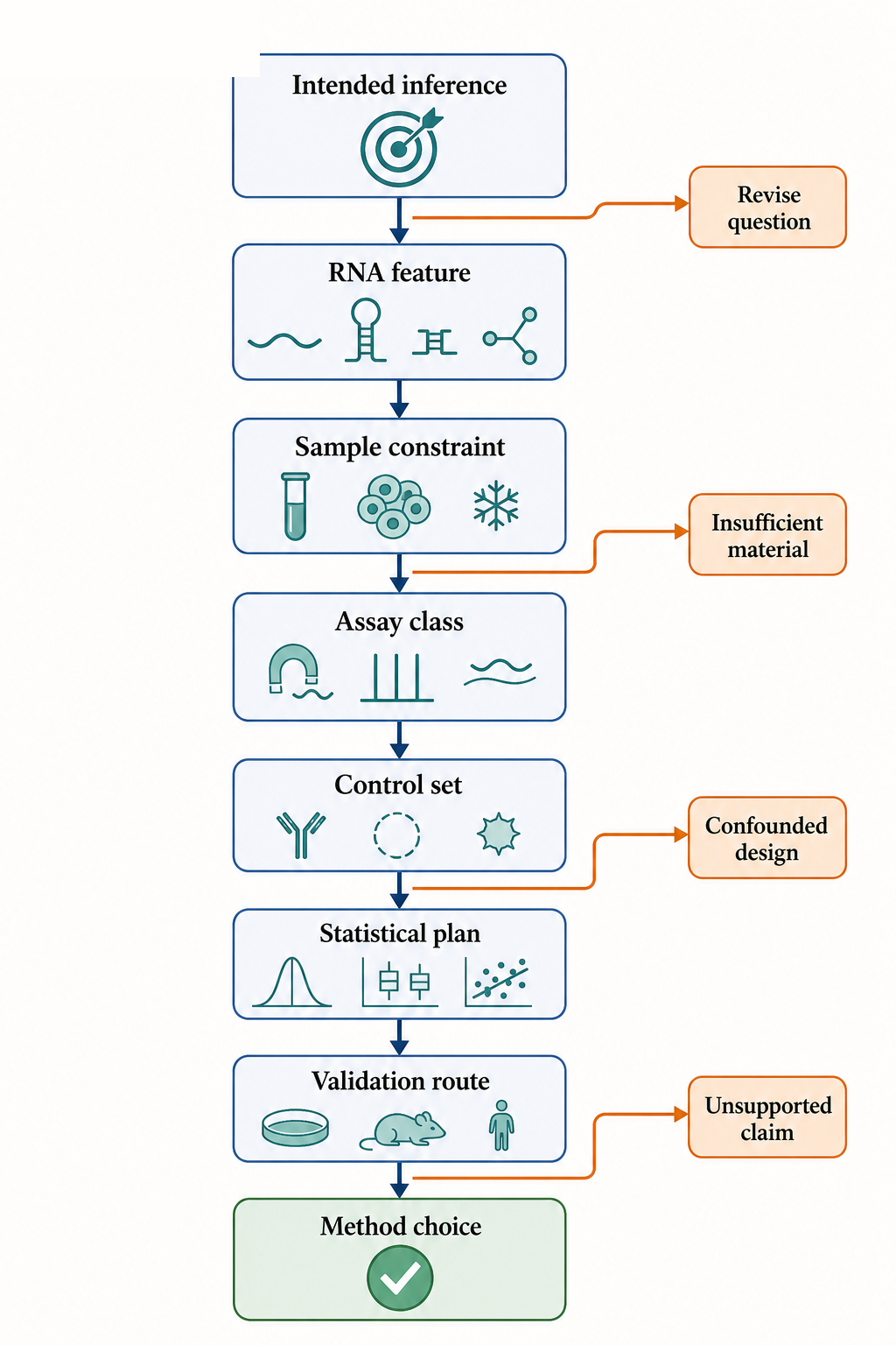
Figure 139.6. Method-Selection Decision Tree for RNA Measurements. Method selection begins with the intended inference, then matches the RNA feature, sample constraints, assay chemistry, design, controls, statistics, and validation evidence.
For translation, ribosome profiling reports ribosome-protected fragments and can reveal translated open reading frames, pausing, frame choice, and translational efficiency when paired with RNA-seq. It does not directly measure completed protein output. Reporter assays test regulatory elements but may lose native context. Proteomics supplies protein-level evidence with different dynamic range and timing. Strong translation claims often combine these evidence types.
For perturbation and causality, RNAi, CRISPR interference, CRISPR activation, CRISPR knockout, base editing, RNA-targeting CRISPR systems, antisense oligonucleotides, splice-switching oligonucleotides, and degron-based protein perturbations each have different off-target, timing, dosage, and mechanism profiles. RNAi can produce partial knockdown and seed-mediated off-target effects. CRISPR knockout can trigger compensation or select for surviving clones. CRISPR interference and activation depend on chromatin context and guide position. Antisense oligonucleotides can alter splicing, degradation, or steric access depending on chemistry and design. A causal claim is stronger when independent reagents, rescue experiments, dose response, temporal order, and orthogonal readouts agree.
Method selection also includes a validation plan. Discovery methods generate candidates; validation methods test whether candidates survive a different measurement principle. Bulk RNA-seq candidates can be validated by RT-qPCR, digital PCR, targeted sequencing, or RNA fluorescence in situ hybridization depending on the claim. Single-cell cluster markers can be validated by imaging, flow cytometry, spatial localization, or independent cohorts. CLIP targets can be validated by mutating binding motifs, perturbing the RNA-binding protein, reporter assays, or biochemical binding. RNA structure models can be validated by compensatory mutations, orthogonal probing reagents, structural biology, or ligand-response experiments. RNA modification calls can be validated by enzyme perturbation, chemical standards, mass spectrometry, or orthogonal sequencing chemistry.
Cost and feasibility are legitimate design variables, but they should be made explicit. A limited budget may support a smaller number of carefully replicated conditions rather than many underpowered contrasts. Rare tissue may require a staged design: pilot assay optimization in abundant material, then focused measurement in rare samples. Degraded archival RNA may make long-read full-length transcriptomics unrealistic but support targeted short-amplicon assays or single-nucleus approaches. A time-sensitive infection experiment may prioritize robust sampling and metadata over maximal molecular breadth. The best method is the method that answers the defined question with acceptable uncertainty under real constraints.
Decision trees should not become rigid recipes. Methods evolve, and local expertise matters. The durable principle is that the method must match the inferential target, and every method choice should be paired with design, controls, statistics, metadata, benchmark awareness, and validation. A reader who asks “What exactly would this result prove, and what could still explain it artifactually?” will choose better RNA methods than a reader who asks only “Which assay is most advanced?”
Box 139.3. A Manuscript Review Checklist for RNA Methods
Ask whether the inferential target is explicit and whether the design uses the correct independent biological unit. Check randomization, blocking, batch balance, artifact-specific positive and negative controls, effect sizes, uncertainty, multiple-testing correction, and power. Require enough metadata and workflow provenance to reproduce the analysis, and confirm that benchmark claims stay within the tested organisms, samples, assays, and tasks. Finally, separate what the assay directly measures from the biological mechanism being claimed and look for orthogonal validation through a different measurement principle.
Recent Consensus
Current practice across RNA methods converges on several principles. Biological replication must match the inferential unit, and technical replication cannot replace it. Randomization, blocking, balanced batch structure, artifact-specific controls, multiple-testing correction, effect sizes, uncertainty, metadata, provenance, realistic benchmarks, negative controls, and orthogonal validation are all parts of reliable RNA evidence.
Open Questions, Controversies, Deprecated Models, and Common Misconceptions
Open questions:
- Several practices remain unsettled or context-dependent. Donor-level modeling in single-cell, multiomic, and spatial datasets is still evolving. Batch correction remains a tradeoff between removing technical variation and preserving biology. RNA modification detection and direct RNA sequencing need stronger chemical validation, error models, and benchmarks. Machine-learning methods require benchmarks that prevent leakage and test generalization across organisms, tissues, RNA families, and laboratories.
Common misconceptions:
- “More cells do not necessarily mean more biological replicates.” More sequencing does not fix confounding.
- “Spike-ins do not automatically normalize global shifts.” A low FDR does not prove mechanism. A public dataset is not automatically FAIR. A negative result is not uninterpretable if the study was powered and controlled for a defined effect. A method that performs best on one benchmark is not universally best. A statistical batch correction cannot recover information that was never collected.
Deprecated or weakened claims:
- Universal housekeeping genes, technical replicates treated as biological independence, fold-change-only differential expression, antibody enrichment as proof of modification, CLIP binding as automatic regulation, and visually separated dimension-reduction clusters as automatic cell types.