Chapter 141. Transcriptome Assembly, Isoform Quantification, Splicing Analysis, and Annotation Updating
Scope Note
This chapter explains how RNA sequencing data are turned into transcript models, isoform abundance estimates, splicing interpretations, allele-aware expression calls, RNA-editing-aware analyses, and updated annotations. The chapter focuses on computational reasoning rather than wet-lab library construction, which is covered in Chapters 125 and 128. The emphasis is on what the inferred RNA objects physically represent, why inference is ambiguous, how evidence should be combined, and how transcript annotations can be updated reproducibly without confusing discovery, quantification, and curation.
Executive Summary
Transcriptome assembly asks which RNA molecules were present in a sample and how their exons, splice junctions, transcription start sites, and 3′ ends were connected. Reference-guided assembly uses a genome and often an existing annotation to order the evidence, whereas de novo assembly reconstructs transcript sequences without relying on a genome. Short reads provide depth and mature statistical tooling but rarely observe complete isoforms directly. Long reads can span full transcript molecules and reveal exon connectivity, yet they still require careful correction for coverage bias, incomplete cDNA synthesis, internal priming, sequencing errors, and library artifacts. The evidence object is therefore not “the transcriptome” itself but a set of reads, alignments, junctions, termini, and compatibility relationships that support transcript models with different degrees of confidence.
Isoform quantification estimates transcript abundances from reads that may be compatible with several transcripts. Ambiguity is not a minor nuisance; it is a central property of transcriptomics whenever isoforms share exons, paralogous genes share sequence, repeats are transcribed, or reads are shorter than the molecules being measured. Modern quantifiers summarize ambiguity through equivalence classes or transcript compatibility classes and often infer abundance by likelihood-based or expectation-maximization procedures. Gene-level counts are usually more stable than transcript-level counts, but gene-level aggregation can hide isoform switching and alternative promoter, splice, and polyadenylation choices.
Splicing analysis can be framed as event-level analysis, transcript-level analysis, or splice-graph analysis. Event-level metrics such as percent spliced in (PSI) can be interpretable when the biological question is a cassette exon, intron retention event, alternative splice site, or mutually exclusive exon pair. Transcript-level interpretation is needed when multiple events occur together on the same molecule, as in many disease-associated isoform switches, long noncoding RNA isoform changes, and circular RNA isoform structures. Long-read sequencing and careful short-read modeling increasingly show that genes can produce coordinated isoform programs rather than independent local events.
Allele-specific expression, RNA editing, and haplotype-aware analysis add another layer: reads must be assigned not only to a gene or transcript but also to a parental haplotype, an allele, or an edited versus genomically encoded state. These analyses are powerful for imprinting, cis-regulatory variation, allele-specific splicing, allele-specific RNA editing, and disease genetics, but they are especially vulnerable to reference bias, mapping ambiguity, low variant density, DNA contamination, and confounding between genomic variants and post-transcriptional edits.
Annotation updating converts computational discoveries into stable reference resources. A robust update workflow separates discovery from curation, records evidence type, grades transcript support, preserves versioned identifiers, removes artifacts, and keeps reproducible pipelines for alignment, assembly, quantification, quality control, and release. The current consensus is that no single technology defines a transcript annotation. Short reads, long reads, cap and poly(A) evidence, proteogenomics, conservation, RNA modification or editing maps, and biological replication each contribute different evidence classes.
Concept Inventory
- Transcript model: a representation of an RNA molecule’s genomic origin and structure, usually including exons, introns removed by splicing, strand, and sometimes transcription start and end sites. A transcript model is an inference from evidence, not direct proof that every modeled molecule exists in every sample.
- Isoform: one transcript variant from a gene or locus. Isoforms may differ by exon inclusion, splice sites, promoter use, 3′ end formation, retained introns, coding sequence, untranslated regions, or noncoding status. Do not restrict “isoform” to protein-coding differences.
- Reference-guided assembly: transcript reconstruction that uses a genome sequence and splice-aware read alignments. Existing annotations may constrain or seed the assembly, but the output can include novel transcript models.
- De novo transcript assembly: reconstruction of transcript sequences from read overlaps or k-mers without requiring a genome. It is essential for non-model organisms, mixed communities, and poorly assembled genomes, but it complicates isoform resolution, paralog separation, and genomic interpretation.
- Equivalence class or transcript compatibility class: the set of transcripts that a read or fragment could have originated from, given sequence, alignment, fragment length, strand, and library assumptions. Equivalence classes make ambiguity explicit rather than forcing a single arbitrary assignment.
- Splice graph: a graph representation in which exons or splice sites are nodes and splice junctions are edges. Splice graphs are useful for assembling transcripts and defining local splicing events, but not every path in a graph is necessarily a real RNA molecule.
- Percent spliced in (PSI): the estimated fraction of transcripts from a locus or local event that include a particular exon, splice junction, or intron-retention state. PSI is a local usage measure, not necessarily a full-transcript abundance measure.
- Allele-specific expression: unequal RNA output from two alleles of the same gene in a diploid or polyploid genome. The cause may be imprinting, cis-regulatory variation, allele-specific chromatin, nonsense-mediated decay, allele-specific splicing, or technical bias.
- RNA editing: a post-transcriptional sequence change in RNA relative to the genomic template, such as adenosine-to-inosine editing detected as A-to-G mismatches in cDNA. RNA editing must be distinguished from DNA variants, sequencing errors, and mapping artifacts.
- Annotation update: a controlled change to a transcript annotation resource, including addition, revision, retirement, or reclassification of transcript models. Annotation updating is a curation process, not merely a command that merges all assembled transcripts.
What to Know Before Reading This Chapter
Readers should understand the basic layout of a eukaryotic gene: a genomic locus has a strand, exons, introns, promoters, transcription start sites, splice donor and acceptor sites, coding sequence, untranslated regions, and 3′ end formation sites. Chapters 18, 27, 28, and 29 provide the underlying gene-model and RNA-processing background. Readers should also know that RNA-seq reads are sampled fragments of RNA-derived molecules rather than a complete census of intact transcripts. Chapter 125 covers how library design, fragmentation, reverse transcription, priming, amplification, strandedness, and depth affect what evidence is available. Chapter 128 covers long-read transcriptomics, including full-length cDNA and direct RNA approaches.
This chapter uses five running examples. First, a protein-coding gene with two cassette exons illustrates the difference between local splicing events and full transcript isoforms. Second, the long noncoding RNA NEAT1 illustrates how isoform balance can carry biological meaning beyond total gene expression; Zakutansky et al. (2024) connect NEAT1 isoform regulation by QKI to glioma transcriptome effects and cell migration. Third, a newly sequenced organism illustrates why de novo transcript assembly remains important when genome annotation is incomplete. Fourth, circular RNA isoform assembly illustrates why ordinary linear transcript assumptions can fail; Wu et al. (2019) developed CircAST for full-length circular RNA isoform assembly and quantification. Fifth, allele-aware analysis illustrates why the same read can carry evidence about expression, splicing, inherited genotype, and editing state.
141.1. Reference-guided and de novo transcript assembly
Transcriptome assembly is the process of reconstructing RNA transcript structures from sequencing evidence. The word “assembly” can be misleading because it suggests that the computational task simply puts observed pieces back together. In practice, most RNA-seq datasets observe incomplete, biased, and uneven pieces of RNA molecules. The algorithm must infer which exons are connected, which splice junctions belong to the same transcript, where transcripts start and end, and which candidate paths are likely to be real rather than products of noise. The central object is therefore an evidence-supported transcript model, not a photograph of the transcriptome.
Reference-guided transcript assembly begins with a genome sequence. Short reads or long reads are aligned to the genome with methods that can represent introns as gaps between exons. A splice-aware alignment of a short read may show that one end maps to the end of exon 2 and the other end maps to the start of exon 3, thereby supporting a splice junction. Paired-end reads add fragment-level constraints because the two read mates should have a plausible orientation and distance. Stranded libraries add strand constraints, reducing confusion between sense and antisense transcription. Existing annotations can be supplied as guides, allowing the assembler to recover known models and focus novelty calls on evidence not explained by existing transcripts. Trapnell et al. (2010) established a landmark reference-guided framework for transcript assembly and quantification by RNA-seq and showed how unannotated transcripts and isoform switching could be detected during cell differentiation.
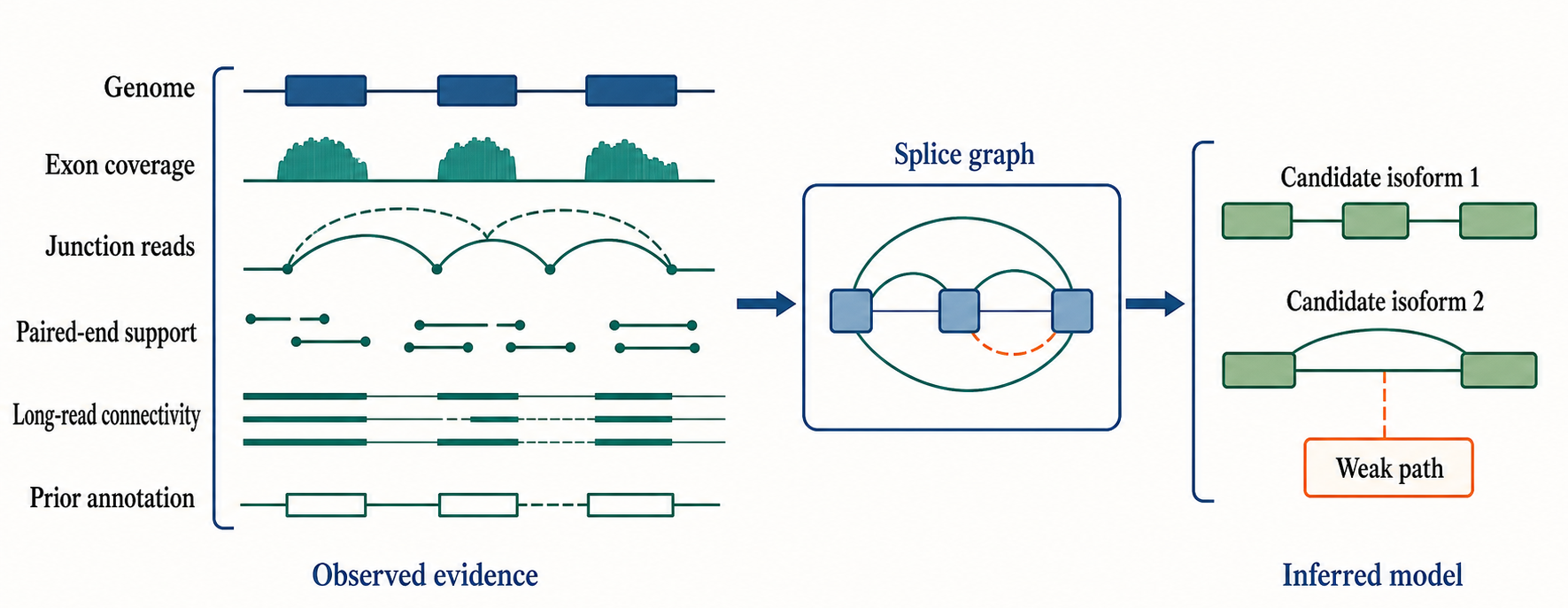
Figure 141.1. Reference-guided transcript assembly from read evidence to transcript models. Reference-guided transcript assembly begins with a genome coordinate system and RNA-seq evidence. Exon coverage, splice-junction reads, paired-end constraints, strandedness, long-read connectivity, and existing annotation support candidate transcript paths. The figure should visually separate observed evidence from inferred transcript models.
The mechanistic logic of reference-guided assembly has several steps. First, reads are aligned and grouped into genomic loci. Second, splice junctions, exon coverage blocks, transcriptional boundaries, and read-pair constraints are converted into a graph or comparable representation. Third, candidate transcript paths through the graph are proposed. Fourth, paths are filtered, merged, or scored by read support, compatibility, abundance, and annotation priors. Fifth, the resulting transcript models are reported in a structured format such as GTF or GFF3, often with confidence attributes. Each step can change the biological interpretation. For example, a weakly covered retained intron can represent a regulated nuclear-retained isoform, a pre-mRNA contamination signal, an unspliced nascent transcript, or a mapping artifact in a repetitive region.
Short-read assembly is powerful because short-read RNA-seq can be deep, inexpensive relative to long-read sequencing, and available across thousands of biological conditions. Depth helps detect low-abundance junctions and supports statistical comparisons across samples. Yet short reads rarely connect distant exons on the same molecule. If exon 2 and exon 5 are both alternatively spliced, reads supporting exon 2 inclusion and reads supporting exon 5 skipping may not reveal whether those choices occur on the same transcript molecules. Paired-end reads help only within the fragment length distribution. This limitation matters for protein isoform prediction, nonsense-mediated decay prediction, long noncoding RNA isoform biology, and therapeutic splice-switching design.
Long-read transcriptomics changes the evidence structure by sequencing much longer cDNA molecules or native RNA molecules. Long reads can connect multiple splice junctions across a transcript and may observe complete or near-complete isoforms. Bayega et al. (2018), Oikonomopoulos et al. (2020), and Tan et al. (2026) review the movement toward single-molecule and long-read transcript profiling, including its relevance for mRNA analysis and disease-associated splicing complexity. A long read spanning a full NEAT1 isoform or a disease-relevant transcript can answer a question that short reads can only model indirectly: which exons, termini, and sequence variants coexist on one molecule?
Long reads do not remove the need for inference. Complementary DNA protocols can truncate molecules during reverse transcription or template switching. Direct RNA sequencing avoids cDNA synthesis but has its own throughput, error, and end-detection limitations. Long-read alignments can be affected by higher per-read error rates, homopolymer errors, paralogous sequence, repetitive exons, and alignment choices near splice junctions. Coverage is often lower than in short-read datasets, so rare isoforms may be missed, and observed singleton transcript models may be difficult to distinguish from artifacts. A careful long-read assembly workflow therefore includes read-quality filters, splice-junction polishing, comparison with short-read junction support, terminal-site evidence, and biological replication.
De novo transcript assembly reconstructs transcript sequences without using a genome as the primary coordinate system. The usual short-read strategy builds a de Bruijn graph from k-mers, traverses paths corresponding to transcript sequences, and estimates which paths are supported by read coverage. This approach is indispensable for organisms without high-quality genomes, mixed species samples, environmental transcriptomes, and historical datasets where the genome is unavailable or fragmented. It can also help discover transcripts absent from a reference genome assembly. The output, however, is a transcript sequence collection rather than a genome-anchored annotation. Downstream interpretation usually requires mapping assembled contigs back to a genome, predicted proteins, transcript databases, or homologous sequences.
The central challenge in de novo assembly is separating biological isoforms from repeats, paralogs, alleles, and graph tangles. A recent gene duplication can produce two highly similar transcripts; a de novo assembler may collapse them into one contig, split one gene into multiple partial contigs, or produce chimeric paths. Heterozygosity can produce allele-specific contigs that are mistaken for paralogs. Alternative splicing can create graph branches that are hard to traverse correctly when isoforms share most exons. Uneven coverage across transcripts can cause low-coverage ends to drop out. For organisms with high repeat content or large gene families, de novo transcriptomes should be treated as useful working resources rather than finished annotations unless they are supported by genome anchoring and independent evidence.
Reference-guided and de novo assembly are not competing philosophies so much as different responses to different evidence states. A high-quality mammalian genome with mature annotation favors reference-guided discovery, annotation augmentation, and conservative novelty classification. A non-model plant, protist, fungus, or symbiotic community may require de novo transcript sequence reconstruction before gene models can be improved. A draft genome can benefit from both: de novo contigs can identify missing exons or misassembled loci, while genome-guided alignments can order and orient transcript evidence. Ringeling et al. (2022) illustrate how changing the input organization of short-read RNA-seq data, in that case by partitioning RNAs by length, can improve reconstruction, reminding readers that assembly quality depends on sample and molecule-class properties as well as on the assembler.
Table 141.1. Assembly strategy comparison. Transcriptome assembly strategies differ in input requirements, strengths, and failure modes. Strategy choice should follow genome quality, annotation maturity, molecule topology, read length, and biological question.
| Strategy | Primary input | Best use case | Main strengths | Common artifacts | Evidence needed before annotation release |
|---|---|---|---|---|---|
| Reference-guided short-read assembly | Splice-aware short-read alignments, paired-end constraints, strandedness, genome, existing annotation | Mature genome with incomplete or condition-specific transcript annotation | Deep junction support, reproducible locus-level coverage, direct integration with genome coordinates and GTF/GFF3 records | Fragmented isoforms, false retained introns, weak terminal boundaries, reference bias, multimapping in repeats or paralogs | Independent junction support, strand consistency, coverage compatible with the model, artifact filtering, replication or orthogonal support |
| De novo transcript assembly | Short-read overlaps or k-mers without requiring a genome | Non-model organisms, mixed communities, missing genomes, fragmented genome assemblies | Recovers transcript sequences when genome coordinates are absent or unreliable; can reveal missing loci | Collapsed paralogs, split isoforms, allele-specific contigs mistaken for genes, chimeric graph paths, lost low-coverage ends | Genome anchoring or homology assignment where possible, read support across contigs, paralog checks, coding or noncoding classification, reproducible detection |
| Hybrid genome-guided and de novo assembly | Draft genome alignments plus de novo transcript contigs and annotation comparison | Draft genomes, incomplete gene models, organisms with missing exons or misassembled loci | Uses de novo contigs to find missing transcript sequence while using the genome to order and orient evidence | Duplicated models, conflicting coordinates, contigs mapped to paralogous loci, overmerging of discovery evidence | Coordinate reconciliation, duplicate collapse, relation-to-annotation categories, splice and terminal support, release-level curator review |
| Long-read-first isoform discovery | Full-length or near-full-length cDNA reads, direct RNA reads, splice polishing, optional short-read support | Genes where exon connectivity, transcript ends, haplotypes, or disease isoforms must be connected on one molecule | Observes multi-exon connectivity and sometimes complete isoforms; can phase variants and splice choices | Truncated cDNAs, template switching, internal priming, lower depth, per-read errors, singleton transcript models | Read-quality filters, polished splice junctions, terminal-site checks, short-read or targeted validation, biological replication before stable release |
| Molecule-class-aware assembly | RNA fractions or protocols matched to molecule class, such as length-partitioned RNA or retained-intron-enriched data | Transcript classes with unusual length, processing, nuclear retention, or coverage profiles | Reduces masking of one molecule class by another and can improve recovery of weak or atypical transcripts | Fraction-specific bias, overinterpretation of enrichment, sample-preparation artifacts, incomplete comparability across datasets | Protocol metadata, fraction-aware thresholds, comparison with unfractionated data, class-specific artifact controls |
| Circular-RNA-specific assembly | Back-splice junction reads, full-length circular isoform evidence, circular-aware alignment or assembly | Circular RNAs and alternatively spliced circular isoforms | Matches non-linear molecule topology and can resolve internal exon composition beyond a back-splice junction | False back-splices, template switching, linear transcript contamination, incomplete circular isoforms | Back-splice support, full-length circular structure when possible, linear-RNA controls, internal exon validation, circular-specific annotation handling |
Circular RNAs are a boundary case that exposes assumptions built into ordinary transcript assembly. A circular RNA is produced by back-splicing, in which a downstream splice donor is joined to an upstream splice acceptor. Standard linear transcript assemblers may discard or misrepresent this evidence because genomic coordinates are expected to proceed monotonically. CircAST, described by Wu et al. (2019), addresses full-length assembly and quantification of alternatively spliced circular RNA isoforms. The important general lesson is that transcript assembly must match the topology of the molecule being modeled. Linear mRNA, retained-intron RNA, fusion RNA, circular RNA, viral RNA, and organellar RNA can require different assumptions.
Evidence standards should be explicit. A high-confidence novel transcript model usually has multiple independent supporting reads, splice junctions with canonical or biologically plausible motifs, strand consistency, coverage compatible with the transcript structure, terminal evidence where possible, absence of obvious mapping artifacts, and reproducibility across biological samples or orthogonal technologies. A lower-confidence candidate may still be valuable as a discovery lead, especially for rare cell types or poorly annotated organisms, but it should not be promoted silently into a reference annotation. Curation-deferred source need: add chapter-local citations for specific assembly software comparisons, GTF/GFF3 validation standards, and community annotation evidence codes.
Box 141.1. Transcript Model, Molecule, or Artifact?
When evaluating a novel transcript model, separate three claims.
- Structure claim: reads support a specific exon, junction, terminal site, or full-length path.
- Molecule claim: an intact RNA carrying that structure exists in the sampled cells.
- Function claim: the RNA has a regulatory, coding, structural, disease, or evolutionary consequence.
The evidence ladder is not automatic. A junction read supports splice-site use, but it does not prove a complete isoform. A long read can support exon connectivity, but a singleton read may still reflect truncation, template switching, or alignment error. High coverage over shared exons supports locus expression more than it supports one particular isoform. Annotation release should therefore record which claim is supported and which remains provisional.
The cross-chapter handoff is direct. Chapter 18 explains how transcript models are represented in browsers and annotation versions. Chapter 125 explains why library construction determines the read evidence available for assembly. Chapter 128 provides deeper treatment of full-length and direct RNA technologies. Chapter 139 explains statistical design and reproducibility expectations for RNA methods.
141.2. Isoform quantification, equivalence classes, and ambiguity
Isoform quantification asks how much RNA came from each transcript model. This question is harder than gene-level counting because many isoforms share sequence. A read from a constitutive exon may be compatible with every annotated isoform of a gene. A read crossing a splice junction may distinguish one subset of isoforms but not another. A read in a repeated exon or duplicated gene family may be compatible with multiple genes. The computational task is therefore not simply counting reads assigned to transcripts; it is estimating transcript abundances from partial and ambiguous evidence.
The most important term is compatibility. A read or fragment is compatible with a transcript if the sequence, orientation, splice pattern, fragment length, and library design are consistent with origin from that transcript. In a gene with three isoforms, a read from exon 1 might be compatible with all three, whereas a read spanning exon 2 to exon 4 might be compatible only with the isoform that skips exon 3. Quantifiers often group reads into equivalence classes, also called transcript compatibility classes, where each class contains reads compatible with the same set of transcripts. These classes are useful because they preserve the structure of ambiguity. They prevent the false precision that would come from assigning every ambiguous read to one transcript before statistical modeling.
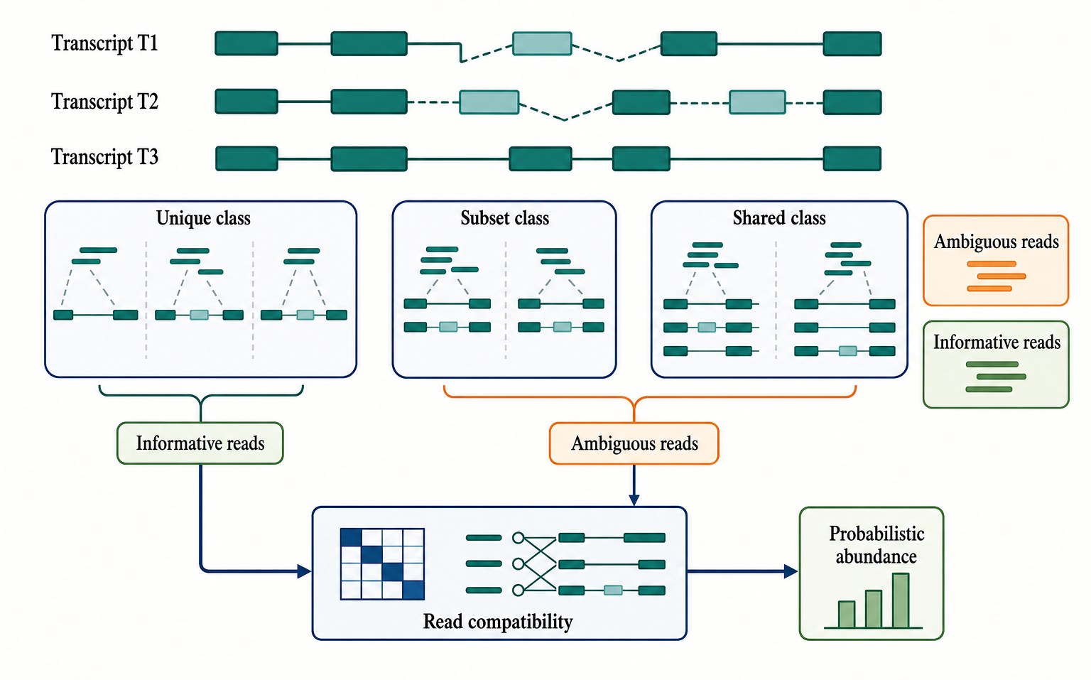
Figure 141.2. Equivalence classes in isoform quantification. Isoform quantification does not assign every read to one transcript before modeling. Reads are grouped by the set of transcripts with which they are compatible. Unique reads provide direct evidence for one isoform, whereas shared reads contribute probabilistically to transcript abundance estimates.
Most isoform quantification methods have the same conceptual workflow. First, a transcript reference is defined, usually from an annotation, an assembly, or a combined reference. Second, reads are aligned, pseudoaligned, or otherwise matched to possible transcripts. Third, fragment-level or read-level compatibility information is summarized. Fourth, a statistical model estimates transcript abundances, frequently using an expectation-maximization-like procedure that distributes ambiguous evidence according to the current abundance estimates and iteratively updates those estimates. Fifth, uncertainty is assessed by bootstrap, posterior sampling, replicate-level modeling, or downstream differential transcript usage methods. Tool-specific details vary, but the biological question is stable: what transcript mixture best explains the observed data under the model assumptions?
Ambiguity has biological and technical sources. Alternative splicing creates shared exons. Alternative transcription start sites and alternative polyadenylation create isoforms that differ only at the ends, which may be poorly covered in fragmented RNA-seq. Gene families and pseudogenes create near-identical sequence. Repeats can produce reads with many genomic placements. Allelic variation can make reads fit a personalized haplotype better than the reference. RNA editing can introduce apparent mismatches. Library biases can make some transcript regions overrepresented or underrepresented. Fragment length distribution affects which isoform differences can be observed. Strandedness determines whether antisense transcripts can be separated from sense transcripts. These sources of ambiguity should be reported, not hidden.
Gene-level counts are often more robust because reads from shared exons can be summed over all isoforms of a gene. That robustness is useful for many differential expression analyses. The cost is loss of transcript-level interpretation. A gene can have unchanged total expression while switching from a coding isoform to a retained-intron isoform, from a long 3′ untranslated region to a short 3′ untranslated region, or from one protein-coding isoform to another with a different domain. Trapnell et al. (2010) highlighted isoform switching during cell differentiation, an example of why abundance at the gene level and abundance at the isoform level answer different biological questions.
Long-read data can reduce ambiguity by observing more exon connectivity per molecule. If a read spans a transcript from the first exon to the poly(A) tail, isoform assignment becomes direct for that molecule. In practice, long-read quantification must correct for lower depth, length-dependent capture, truncated reads, variable read quality, and molecule-specific biases. A long-read dataset may be excellent for discovering transcript structures but underpowered for precise abundance estimation, especially for low-expression isoforms. Hybrid strategies can use long reads to define isoform models and short reads to quantify those models, but the hybrid approach inherits assumptions from both technologies.
Table 141.2. Sources of ambiguity in isoform quantification. Isoform quantification ambiguity arises from shared exons, duplicated sequence, incomplete transcript boundaries, library bias, variant differences, editing, and reference incompleteness. Each ambiguity source suggests a different control or validation strategy.
| Ambiguity source | Example | Effect on quantification | Mitigation | Residual caveat |
|---|---|---|---|---|
| Shared exons among isoforms | Constitutive exon reads compatible with every transcript from a gene | Abundance is redistributed by the model rather than directly observed for each isoform | Use junction-informative reads, paired-end geometry, equivalence classes, uncertainty estimates, and replication | Isoforms with little unique sequence can remain weakly identifiable even at high gene expression |
| Coupled distant splicing events | Exon 2 inclusion and exon 5 skipping occur in the same gene but outside one short fragment | Local evidence cannot prove which choices occur on one RNA molecule | Add long-read, targeted, or paired-end evidence that connects events; report event-level and transcript-level results separately | Long-read depth may be too low for precise abundance estimates |
| Alternative transcript ends | Isoforms share internal exons but differ at promoter or polyadenylation sites | Short fragmented reads may collapse regulatory end variants or split them artificially | Use cap, 5′ end, poly(A)-site, 3′ end, or full-length evidence when end usage is the question | End-capture protocols have their own priming, truncation, and internal-priming artifacts |
| Paralogous genes, pseudogenes, and repeats | Reads map equally well to related loci or low-complexity sequence | Reads can be assigned to the wrong transcript, gene, or locus | Require mapping-quality filters, multimapping-aware models, unique sequence, and genome-assembly review | Recently duplicated or poorly assembled regions can remain unresolved |
| Allelic variation and reference bias | Alternate-allele reads align less efficiently than reference-allele reads | Transcript or allele abundance can be biased toward the reference representation | Use variant-aware alignment, masked heterozygous sites, personalized or haplotype-resolved transcript references | Sparse informative variants limit allele-aware quantification |
| RNA editing and RNA-DNA mismatches | A-to-I editing appears as an A-to-G difference in cDNA-based data | Edited reads may be confused with variants, errors, or mismapped paralogs | Use matched DNA or variant filters, strand-aware analysis, repeat-aware mapping, and site-level coverage thresholds | Editing level and isoform abundance can be confounded without phased or molecule-level evidence |
| Library and molecule bias | Fragment length, strandedness, degradation, truncation, or length-dependent capture changes read distribution | Some transcript regions or isoform classes are overrepresented or underrepresented | Model fragment length and strandedness, inspect coverage, compare protocols, and validate key isoforms orthogonally | Bias correction cannot recover evidence for molecules the assay rarely captured |
| Annotation incompleteness or overgranularity | Adding a novel isoform creates new compatibility classes; splitting weak end variants adds artificial choices | Estimated abundance changes when the transcript reference changes | Record annotation version, compare old and new references, filter weak models, and run regression checks | Quantification remains conditional on the chosen transcript reference |
Equivalence classes also shape downstream statistical testing. A transcript with many unique reads has stronger abundance evidence than a transcript whose estimated abundance is driven mostly by reads shared with a highly expressed isoform. Differential transcript usage analysis should distinguish changes supported by isoform-informative reads from changes inferred indirectly because another transcript changed. For example, if isoform A and isoform B share most sequence and only isoform B has a unique junction, an apparent decrease in isoform A may be a statistical consequence of increased evidence for isoform B. That inference can be valid under the model, but it should be interpreted as model-based and tested against biological replication.
Transcript length normalization is another point where vocabulary matters. Counts, transcripts per million (TPM), fragments per kilobase per million (FPKM), and related measures do not mean the same thing. Raw or estimated counts are closer to the number of observed fragments assigned to a transcript and are often used for statistical modeling. TPM normalizes for transcript length and library size and is useful for within-sample comparisons of relative transcript abundance. FPKM and related measures historically served similar roles but have limitations for cross-sample inference. A longer transcript has more positions from which fragments can be sampled, so length adjustment is needed when comparing transcript concentration rather than read yield. However, length normalization can be misleading when transcripts are partially degraded, incompletely covered, or incorrectly annotated.
Box 141.2. Reading TPM Without Overreading It
Transcripts per million (TPM) is useful for asking which modeled transcripts are relatively abundant within a sample after length and library-size normalization. It is not an absolute molecule count, and it is not independent of annotation. If a new isoform is added to the transcript reference, ambiguous reads may be redistributed and TPM values for older isoforms can change. If a transcript boundary is wrong, the effective length used for normalization can also be wrong.
Use TPM for descriptive within-sample abundance patterns, but use appropriate count-based or replicate-aware models for differential testing. Treat low-TPM estimates cautiously when they depend on few informative reads. Treat high-TPM estimates cautiously when most support comes from exons shared by several isoforms. Always report the annotation release, quantifier, library type, and uncertainty summary when making transcript-level claims.
Spliced transcript quantification also interacts with transcript boundaries. Two isoforms may have identical internal exon structure but different transcription start sites or polyadenylation sites. Ordinary short-read RNA-seq may not distinguish those end isoforms unless reads cover the distinguishing regions or specialized end-capture protocols are used. Conversely, a change in 3′ end usage can alter 3′ untranslated region regulatory motifs without changing protein sequence. If the annotation collapses end variants, the quantification result will hide regulatory differences. If the annotation splits poorly supported ends too aggressively, the quantifier may distribute reads across artificial isoforms. Annotation granularity therefore controls the question that quantification can answer.
Do not overgeneralize from high transcript abundance to high confidence in transcript structure. A transcript model can be abundant because reads from shared exons support the locus strongly, while the unique structure of that model remains weakly supported. Conversely, a low-abundance transcript may have a small number of highly informative junction-spanning or full-length reads that support its structure. Confidence in abundance and confidence in structure are related but distinct evidence dimensions.
Isoform quantification is also sensitive to the reference transcriptome. Adding a novel isoform can change estimated abundances of existing isoforms because some reads now have an additional compatible origin. Removing a dubious isoform can redistribute reads to remaining models. This is not a bug; it reflects the conditional nature of abundance estimates. The result of transcript quantification is abundance relative to a specified transcript reference, library model, and statistical model. Chapter 18 discusses annotation versioning, and Chapter 144 discusses data systems needed to record these dependencies.
Current consensus is pragmatic. Use gene-level analysis when the biology or data do not support transcript-level claims. Use transcript-level quantification when isoform differences are central and the annotation, read design, and replication support the question. Use long-read or targeted validation for claims about full-length isoform structure, isoform switching with functional consequences, or clinically relevant transcript usage. Curation-deferred source need: add local references for transcript quantification algorithms, pseudoalignment, uncertainty propagation, and differential transcript usage benchmarking.
141.3. Splicing event analysis and transcript-level interpretation
Alternative splicing is the regulated production of multiple RNA isoforms from a precursor transcript by choosing different splice sites, exons, or intron-retention outcomes. Splicing event analysis reduces this complexity to local patterns such as cassette exon inclusion, alternative 5′ splice site choice, alternative 3′ splice site choice, mutually exclusive exons, and intron retention. This reduction is useful because local events can often be measured with reads that cross diagnostic splice junctions. It is also biologically meaningful because many splicing regulators act by promoting or repressing recognition of nearby splice sites. Chapter 28 covers the molecular regulation of alternative splicing; this section focuses on how computational analysis turns RNA-seq evidence into interpretable splicing claims.
The most common event-level quantity is percent spliced in, abbreviated PSI. For a cassette exon, PSI estimates the fraction of transcripts from the local event that include the exon. Inclusion reads may support junctions from the upstream exon into the cassette exon and from the cassette exon into the downstream exon. Skipping reads support the junction from the upstream exon directly to the downstream exon. The PSI estimate compares inclusion-supporting and skipping-supporting evidence, often with corrections for effective length and read geometry. PSI is attractive because it has a bounded and intuitive scale: zero means complete skipping in the modeled event, and one means complete inclusion.
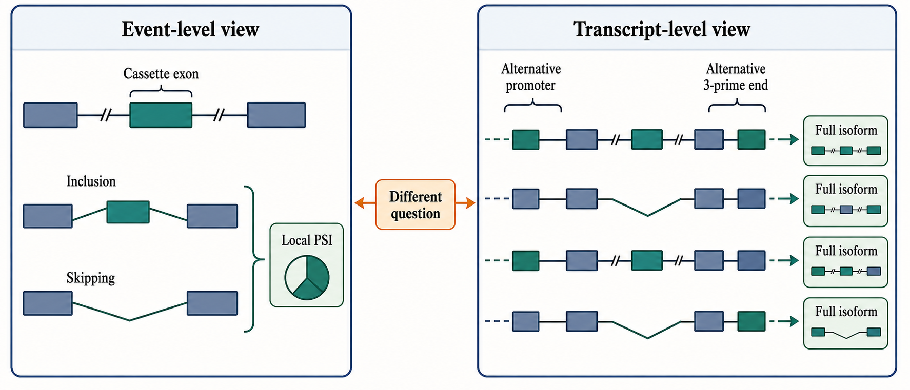
Figure 141.3. Event-level splicing versus transcript-level interpretation. Percent spliced in summarizes local inclusion of a splicing event, but a full RNA molecule can combine that event with other transcript features. Event-level and transcript-level analyses answer different biological questions.
PSI is not a universal measure of transcript function. A local event can occur in several transcript backgrounds. A cassette exon inclusion event may be coupled to an alternative promoter, downstream exon choice, alternative polyadenylation site, or nonsense-mediated decay. If the same cassette exon is included in one full-length isoform and skipped in another, PSI captures local exon usage but not the full molecule. This distinction matters when interpreting protein domains, noncoding RNA scaffolds, localization signals, microRNA target sites, and premature termination codons. A biologically meaningful question may be “is exon 4 included?” or “which complete isoform is produced?” The correct analysis depends on the mechanism under study.
Event definition itself can introduce ambiguity. A complex gene may contain overlapping cassette exons, alternative donor sites, retained introns, and mutually exclusive exons. One algorithm may decompose the locus into several simple events; another may represent the locus as a splice graph; a transcript quantifier may estimate abundance of full transcript models. These frameworks can yield results that are individually valid but not directly interchangeable. A change in a splice junction may appear as a cassette exon event in one representation and as a transcript usage change in another. Readers should ask which event universe was tested and whether the reported event is an independent biological unit or a local summary of a larger isoform change.
Splicing event evidence comes from junction reads, exon-body coverage, intronic coverage, paired-end constraints, full-length reads, and sometimes orthogonal methods such as reverse-transcription PCR, targeted long-read sequencing, or proteomics. Junction reads are strong evidence that two splice sites are joined in at least some molecules. Exon-body coverage alone is weaker because coverage can reflect overlapping transcripts, retained introns, unprocessed RNA, or mapping from homologous sequence. Intronic coverage can indicate intron retention, nascent transcription, slow splicing, nuclear retention, genomic DNA contamination, or annotation problems. Long reads can connect multiple events, but low depth can limit precise PSI estimation. Strong splicing interpretation usually combines local read evidence with transcript context.
Retained introns require special caution. Intron retention can be a regulated mechanism that changes RNA localization, translation, decay, or nuclear detention. It can also arise from incomplete splicing of nascent RNA, contamination by pre-mRNA, inefficient depletion of ribosomal or nuclear RNA, or poor annotation of exons inside a region labeled as intronic. A retained-intron claim is stronger when the RNA is mature enough to have other processed features, the intron-retaining molecule is reproducible, the signal is not explained by nascent RNA enrichment, and the retained region has evidence inconsistent with an unannotated exon or overlapping transcript. Chapter 31 discusses nuclear RNA surveillance and cryptic transcripts, which often complicate intron-retention interpretation.
Alternative splice-site events require resolution at exon boundaries. A shift of a few nucleotides at a donor or acceptor site can alter coding frame, protein motifs, RNA-binding protein motifs, or nonsense-mediated decay. Short reads can detect such shifts when they cross the relevant junction with enough unique anchor sequence. However, alignment near microexons, repeats, or sequencing errors can create false splice-site variation. Microexons are particularly difficult because their small size reduces unique mapping evidence. The computational evidence should therefore include splice motif plausibility, read anchor quality, conservation where relevant, and sensitivity to alignment parameters.
Transcript-level interpretation becomes essential when splicing events are coordinated. A disease-associated splicing regulator may shift many targets, but within one target gene the biologically relevant product may be a full transcript with a specific exon combination. Tan et al. (2026) review long-read sequencing evidence for splicing complexity in human diseases, including the ability of long reads to connect complex isoform structures that short reads fragment into separate events. In cancer or neurodevelopmental disease, an isoform switch may change protein domains, subcellular localization, stability, or noncoding regulatory functions. For lncRNAs, exon connectivity may determine RNP binding, localization, or architectural function rather than protein coding.
The NEAT1 example illustrates the difference between total expression and isoform interpretation. NEAT1 produces isoforms with distinct roles in paraspeckle biology. Zakutansky et al. (2024) report that the RNA-binding protein QKI regulates NEAT1 isoform balance, affects the glioma transcriptome, and impacts cell migration. The computational lesson is that a gene-level NEAT1 count is insufficient if the biological phenotype depends on relative isoform usage. A splicing or isoform analysis must track the relevant transcript forms, estimate their balance, and consider whether the evidence distinguishes isoform-specific effects from total gene expression effects.
Circular RNA splicing further expands the concept of event analysis. Back-splice junction reads indicate circularization, but they do not automatically define the complete circular RNA isoform. A circular RNA can contain alternative internal exons, retained intronic sequence, or multiple back-splice products from the same host gene. Wu et al. (2019) developed CircAST to assemble and quantify alternatively spliced circular RNA isoforms, showing that circular RNA analysis needs full-length isoform reasoning rather than only back-splice detection. For functional interpretation, the question may be whether a circular RNA contains a binding site, open reading frame, structured domain, or regulatory exon, not merely whether a back-splice junction exists.
Table 141.3. Splicing analysis frameworks and interpretations. Splicing analysis frameworks answer different questions. Local event metrics are interpretable for specific splice choices, whereas transcript-level and circular RNA methods are required when exon combinations or molecular topology matter.
| Framework | Evidence object | Best question | Main limitation | Validation approach |
|---|---|---|---|---|
| Event-level PSI analysis | Inclusion and skipping reads for a defined cassette exon, intron-retention event, alternative donor, alternative acceptor, or mutually exclusive exon pair | Did local splice-site or exon usage change between conditions? | Local event usage may not identify the complete transcript carrying the event | Replicated RNA-seq, effect-size and uncertainty reporting, RT-PCR or targeted sequencing for important events |
| Junction-level analysis | Counts for individual splice junctions or junction pairs | Which splice junctions are gained, lost, or differentially used? | A junction read proves a splice connection in some molecules but not a stable full-length isoform | Anchor-quality checks, splice-motif plausibility, mapping-parameter sensitivity, and transcript-context review |
| Transcript-level quantification or differential transcript usage | Estimated abundance of transcript models and their compatibility classes | Did relative isoform use change at a gene or locus? | Estimates depend on annotation completeness, shared reads, library model, and uncertainty treatment | Isoform-informative reads, bootstraps or replicate models, annotation-version reporting, long-read or targeted validation |
| Splice-graph interpretation | Exons, splice sites, or exon segments as nodes and observed junctions as edges | What candidate transcript paths or complex local event structures are supported? | Not every graph path corresponds to an observed RNA molecule | Require path-specific read support, abundance filtering, full-length evidence for complex paths, and artifact review |
| Retained-intron analysis | Intronic coverage, exon-intron junctions, mature-RNA features, and transcript context | Is an intron retained in a processed transcript or is the signal nascent or contaminating RNA? | Intronic signal can reflect pre-mRNA, slow splicing, genomic DNA, unannotated exons, or overlapping transcripts | Nuclear/cytoplasmic context, DNA controls, mature end evidence, reproducibility, and exclusion of alternative annotations |
| Circular RNA isoform analysis | Back-splice junctions plus internal exon composition and circular-aware transcript models | Which circular isoforms, not just which back-splice junctions, are present? | Back-splice detection alone does not define full circular topology or internal splicing | Circular-aware assembly, full-length circular reads when possible, linear-RNA controls, and internal-exon validation |
Differential splicing analysis should be framed around replication and effect size. A statistically significant change in PSI can be biologically small, especially in high-depth datasets. A large PSI shift in a low-expression gene can be unstable if based on few reads. Multiple testing across thousands of events requires correction. Batch effects, cell composition changes, RNA quality, and library differences can mimic splicing differences. For single-cell RNA-seq, sparse coverage usually limits event-level splicing calls except for highly expressed genes or specialized protocols. A strong claim states the event, the transcript or gene context, the tissue or condition, the effect size, the uncertainty, the evidence type, and whether the event was validated.
Common misconceptions deserve explicit correction. A novel junction is not automatically a novel functional isoform. A differential exon signal is not automatically a change in protein abundance. A transcript model containing a premature termination codon is not necessarily degraded unless nonsense-mediated decay is active in that context and the transcript reaches the relevant surveillance machinery. A local splicing event should not be assumed independent of transcription, chromatin, RNA-binding proteins, RNA modification, RNA decay, or translation. Splicing analysis is a bridge between RNA processing mechanisms and transcriptome measurement, not a standalone list of junctions.
The cross-chapter handoff is broad. Chapter 27 explains spliceosome chemistry and splice-site recognition. Chapter 28 develops regulated alternative splicing mechanisms. Chapter 77 covers noncanonical coding potential, which can be affected by isoform choice. Chapter 94 covers circular RNAs. Chapter 128 covers long-read evidence that connects splicing events into full molecules.
141.4. Allele-specific expression, RNA editing, and haplotype-aware analysis
Allele-specific expression analysis asks whether the two alleles of a gene contribute equally to RNA output. In a diploid human cell, one allele may carry a single-nucleotide variant that marks reads derived from that parental chromosome. If heterozygous sites occur inside transcribed regions, RNA-seq reads overlapping those sites can be counted by allele. A balanced gene might show approximately equal maternal and paternal read counts, whereas an imprinted gene, a cis-regulatory variant, an allele-specific splicing event, or nonsense-mediated decay of one allele can create imbalance. The biological object is allele-resolved RNA output, not merely variant calling from RNA.
The simplest allele-specific expression workflow has five steps. First, identify heterozygous variants from matched DNA sequencing or a reliable genotype resource. Second, align RNA reads in a way that minimizes reference bias. Third, count reads overlapping informative heterozygous sites, requiring base quality, mapping quality, and strand consistency. Fourth, test whether observed allelic counts deviate from expected balance while accounting for overdispersion and technical bias. Fifth, interpret imbalance in relation to gene expression, splicing, imprinting, copy number, nonsense-mediated decay, cell type, and disease state. Each step has failure modes.
Reference bias is the central technical problem. Reads carrying the reference allele often align more easily to the reference genome than reads carrying an alternate allele. If the analysis simply maps to a single reference genome, allele-specific expression can be biased toward the reference allele. Variant-aware alignment, masking heterozygous sites, mapping to personalized genomes, or using haplotype-resolved transcript references can reduce this bias. The relevant question is not whether bias has been eliminated absolutely, but whether the workflow has made allelic comparison fair enough for the claimed effect size.
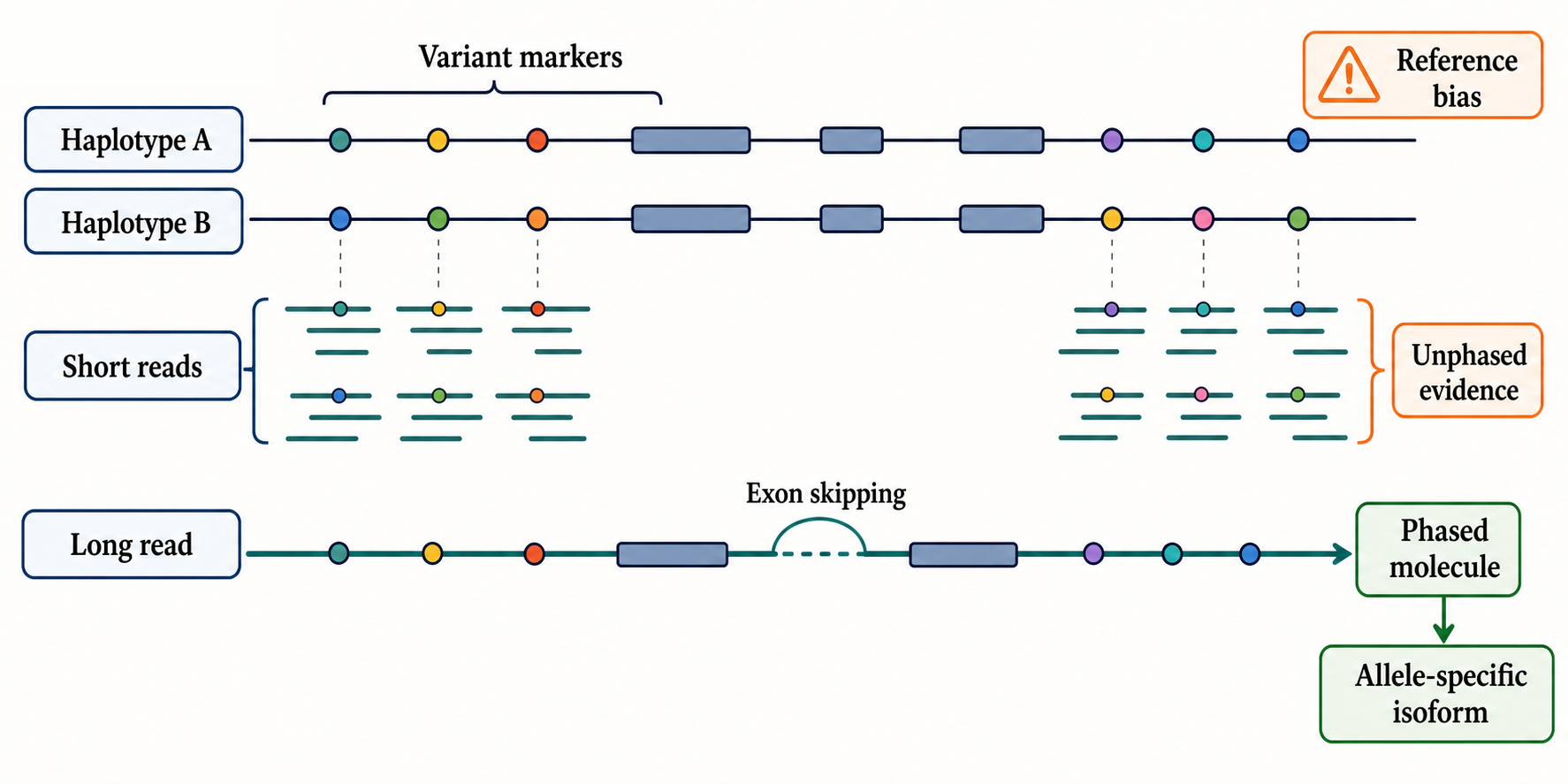
Figure 141.4. Haplotype-aware analysis connects alleles, variants, and splice choices. Haplotype-aware transcriptomics uses inherited variant combinations to assign RNA molecules to parental or population haplotypes. Long reads can connect distant heterozygous variants and splice junctions on one molecule, supporting allele-specific isoform interpretation.
Allele-specific splicing extends allele-specific expression from total output to isoform choice. A variant may disrupt a splice donor, splice acceptor, branch point, exonic splicing enhancer, exonic splicing silencer, intronic regulatory motif, RNA secondary structure, or RNA-binding protein site. The result can be increased exon skipping, intron retention, cryptic splice-site use, or altered transcript stability from one allele. Evidence is strongest when reads connect the allele-marking variant to the splice event on the same molecule. Short reads can do this when the variant and junction occur in the same read or read pair. Long reads can phase distant variants and splice choices across a full transcript, making haplotype-aware isoform analysis especially valuable.
Haplotype-aware analysis assigns reads or transcript models to longer inherited chromosome segments rather than isolated alleles. A haplotype is a set of variants inherited together. Haplotype-aware transcriptomics is useful because a transcript molecule can carry several variants, and the combined pattern can identify its parental or population haplotype. This matters for compound heterozygosity, allele-specific isoform expression, phasing of disease variants with cryptic splicing, and distinguishing paralogous or duplicated loci. In highly polymorphic regions, a haplotype-resolved reference can improve both alignment and transcript quantification.
Long-read sequencing is particularly useful for haplotype-aware transcript analysis because one read can span multiple heterozygous variants and multiple splice junctions. A full-length read may show that haplotype A produces a transcript including exon 6 and haplotype B produces a transcript skipping exon 6. Short-read data might detect allele imbalance at one variant and a splicing change at a junction but fail to prove that they occur on the same molecule. Tan et al. (2026) review how long-read sequencing can reveal disease-relevant splicing complexity; the same evidence structure supports allele-resolved interpretation when informative variants are present.
RNA editing creates a different relationship between RNA sequence and genome sequence. Adenosine-to-inosine editing by ADAR enzymes is often observed in cDNA or RNA sequencing as an A-to-G difference relative to the genome because inosine is read like guanosine during reverse transcription or sequencing interpretation. APOBEC-family cytidine editing can produce C-to-U changes in specific contexts. Chapter 50 covers editing enzymes and biology. Computationally, RNA editing detection must distinguish post-transcriptional changes from inherited DNA variants, somatic DNA variants, sequencing errors, mapping artifacts, and alignment errors in repeats.
RNA editing analysis usually requires matched DNA or a well-curated variant filter. Without DNA evidence, a mismatch in RNA could be a genomic variant. Without careful mapping, apparent editing can arise when reads from a paralog or pseudogene are forced onto a similar reference locus. Without strand awareness, the apparent substitution type can be misread. Without expression and coverage thresholds, random errors can appear as low-level editing. Editing levels can also vary by tissue, developmental state, interferon signaling, RNA structure, and subcellular localization. A strong editing claim states the edited site, genomic context, read support, strand, editing fraction, DNA exclusion evidence, known editing database status if available, and biological condition. Curation-deferred source need: add local references for RNA editing databases, ADAR editing detection benchmarks, and matched DNA/RNA filtering practices.
Allele-specific expression and RNA editing can confound each other. Suppose one allele carries a G at a position where the reference has A, while transcripts from the other allele can be A-to-I edited and read as G. RNA reads with G at that site could come from the genomic G allele or from edited RNA from the A allele. If nearby phased variants are unavailable, the two explanations may be difficult to separate. Conversely, allele-specific editing is biologically real in some contexts: local sequence variants can change double-stranded RNA structure or ADAR access, causing one allele’s transcript to be edited more than the other. Haplotype-aware analysis helps distinguish these cases by using multiple variants along the same molecule.
Allele-specific and haplotype-aware analyses also interact with transcript annotation. A variant inside an exon that exists in one annotation but not another changes which reads are counted as transcript evidence. A retained intron may contain informative variants that improve phasing but also raise the possibility of nascent RNA or pre-mRNA contamination. A novel isoform may place a disease variant in a coding sequence, untranslated region, retained intron, or noncoding RNA that was absent from the old annotation. Annotation updates must therefore record how allele-aware evidence was used and whether a transcript model is supported on one haplotype, both haplotypes, or a population-level consensus.
Population genetics introduces additional cautions. Mapping and annotation resources often represent one reference genome or a small set of haplotypes. Underrepresented populations may have more unmodeled variation relative to the reference, increasing mapping bias and reducing transcript assignment accuracy. Allele-specific results should therefore be interpreted with awareness of ancestry, reference representation, and variant-calling quality. For clinical transcriptomics, a haplotype-aware result can be powerful but should be validated in a diagnostic framework appropriate to the disease, sample type, and regulatory context.
The cross-chapter handoff includes Chapter 50 for RNA editing mechanisms, Chapter 125 for RNA-seq biases, Chapter 128 for long-read phasing, Chapter 139 for statistical design, and Chapter 144 for data systems that can store haplotype-resolved transcript annotations.
141.5. Annotation update workflows and reproducible pipelines
Annotation updating is the process of revising a reference transcript annotation in response to new evidence. It includes adding transcripts, modifying exon boundaries, adding or retiring isoforms, updating biotypes, separating paralogous loci, revising untranslated regions, annotating circular or fusion transcripts in appropriate resources, and changing confidence labels. A reference annotation is a scientific claim set and an infrastructure dependency. Changing it affects read alignment, quantification, differential expression, variant interpretation, genome browser display, knowledge graphs, and downstream clinical or functional conclusions.
A robust annotation update workflow separates discovery from release. Discovery is permissive: it asks what the data might contain. Release curation is conservative: it asks which models should become stable resources. Mixing these stages leads to inflated annotations that include artifacts, sample-specific noise, and redundant transcript fragments. The first stage may assemble all plausible transcripts from multiple datasets. The second stage classifies candidates by relation to known genes, read support, junction confidence, terminal evidence, coding potential, conservation, replication, and artifact risk. The third stage merges accepted changes into a versioned annotation with stable identifiers and change logs.
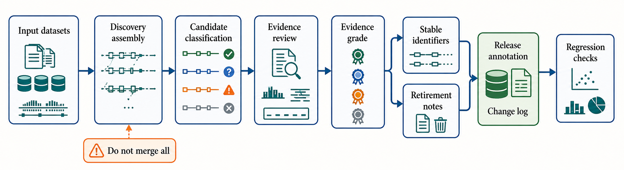
Figure 141.5. Annotation update workflow from discovery to versioned release. Annotation update workflows should separate permissive discovery from conservative release curation. Candidate transcript models are classified, filtered, evidence graded, assigned stable identifiers or retirement notes, and released with versioned change logs.
Evidence classes should be recorded explicitly. Short-read junction support is strong evidence for splice-site use but weak evidence for complete isoform structure. Long-read full-length support is strong evidence for exon connectivity but may be weaker for low-abundance quantification. Cap analysis or 5′ end evidence supports transcription start sites. Poly(A)-site evidence supports transcript ends but must control for internal priming. Proteomics can support coding potential but cannot usually distinguish all RNA isoforms. Conservation can support functional importance but is limited for lineage-specific transcripts. RNA-binding, chromatin, or modification data can support regulatory hypotheses but should not by themselves define transcript structure.
Table 141.4. Evidence classes for annotation updates. No single assay fully defines a transcript annotation. Short reads, long reads, terminal assays, proteomics, conservation, and functional data support different claims about structure, abundance, function, and reproducibility.
| Evidence class | Supports | Does not prove | Artifact controls | Release-use recommendation |
|---|---|---|---|---|
| Short-read junction support | Use of specific splice donor and acceptor sites in at least some molecules | Complete isoform structure, transcript ends, function, or stable abundance | Unique anchors, splice-motif checks, strand consistency, multimapping filters, replicate junction support | Strong support for junction annotation; require additional evidence before adding full novel transcripts |
| Exon and intron coverage | Expression across exonic regions; possible retained introns or unannotated exons | That the covered region is a mature transcript segment or regulated intron-retention isoform | Coverage uniformity checks, DNA contamination controls, nascent-RNA context, overlap with other annotations | Use as supportive evidence, not as sole release evidence for transcript structure |
| Long-read full-length or near-full-length reads | Exon connectivity, candidate isoform paths, termini in favorable protocols, and possible haplotype phasing | Precise low-abundance quantification or broad recurrence across tissues | Read-quality filters, splice polishing, truncation and template-switch controls, singleton review | Valuable discovery and structure evidence; promote only with quality thresholds and replication or orthogonal support |
| 5′ end or cap-associated evidence | Transcription start-site support and promoter-proximal transcript boundaries | Downstream exon connectivity, full transcript abundance, or coding potential | Cap-enrichment specificity, internal priming or degradation checks, strand and replicate consistency | Use to refine starts when compatible with transcript-body evidence |
| Poly(A)-site or 3′ end evidence | Transcript end support and alternative polyadenylation choices | Upstream isoform structure or protein consequence | Internal-priming filters, A-rich genomic context review, degradation checks, protocol metadata | Use to refine transcript ends with explicit internal-priming controls |
| Proteomic or translation-related evidence | Coding potential, translated open reading frames, or peptide-level support for some isoforms | Complete RNA isoform identity or absence of untranslated isoforms | Peptide uniqueness, protein-database versioning, reading-frame consistency, contamination review | Use for biotype and coding-status support, not as sole transcript-structure evidence |
| Conservation or comparative evidence | Evolutionary preservation of sequence, splice sites, or transcript organization | Function for lineage-specific transcripts or expression in the sampled condition | Orthology review, repeat masking, alignment-quality checks, lineage-aware interpretation | Support confidence labels, especially when combined with expression and structure evidence |
| Functional, regulatory, or molecular-context evidence | Association with RNA-binding proteins, chromatin state, modification, localization, phenotype, or perturbation response | Exact transcript boundaries or direct causality by itself | Assay-specific controls, perturbation specificity, independent replication, separation from total gene expression | Use to prioritize and annotate biological relevance after structure evidence is established |
| Biological replication and release regression checks | Recurrence across samples and stability of annotation effects on quantification and identifiers | Mechanism or function of the transcript model | Batch, tissue, cell-composition, and workflow-version controls; old-versus-new annotation comparison | Required for conservative release decisions and for documenting additions, revisions, retirements, and reclassification |
A practical workflow begins with input definition. The curator records genome assembly version, existing annotation version, sample metadata, library protocols, read lengths, strandedness, replicate structure, tissue or cell type, disease state, sequencing technology, and quality thresholds. The workflow then performs quality control, alignment or transcript matching, assembly, quantification, and candidate classification. Candidate transcript models are compared with existing annotation using categories such as exact known transcript, novel combination of known junctions, novel junction, retained intron, antisense transcript, intergenic transcript, possible readthrough, possible fusion, circular candidate, or likely artifact. The exact category names vary across projects, but the principle is stable: relation to existing annotation must be machine-readable and human-auditable.
Reproducibility requires pinned software, parameters, references, containers or environments, workflow definitions, checksums, and reportable quality metrics. A transcript annotation cannot be evaluated if the genome assembly version, splice-aware aligner parameters, assembler version, transcript filters, or merge rules are unknown. Workflow managers and FAIR data systems, discussed in Chapter 144, help make annotation updates repeatable. Chapter 139 provides broader standards for experimental design and reproducibility. Curation-deferred source need: add local references for workflow manager best practices, FAIR transcriptomics standards, and community annotation release policies.
Annotation versioning is not bookkeeping trivia. A gene may have different transcript identifiers, exon coordinates, and biotype classifications across releases. A differential transcript usage result from one annotation may not reproduce under another. A variant described as intronic in an older release may become exonic in a newer release. A lncRNA may be reclassified as a protein-coding transcript if ribosome profiling and proteomics support a translated small open reading frame, or a predicted coding transcript may be reclassified as nonsense-mediated decay candidate. Chapter 18 treats transcript model versioning in detail; the operational point here is that every analysis must record the annotation version used.
Quality filters should target known artifact modes. Internal priming can create false 3′ ends when oligo(dT) priming occurs at internal A-rich sequence. Template switching can create chimeric reads. Genomic DNA contamination can mimic intron retention. Strand-switching or unstranded libraries can confuse antisense transcription. Low-complexity sequence and repeats can produce multimapping reads. Misassembled genome regions can make correct transcript evidence appear inconsistent. Low-level pervasive transcription can generate reproducible but functionally uncertain RNA fragments. A curation workflow should not automatically discard all unusual signals, because some unusual signals are biologically important, but it should label the evidence and require stronger support before release.
Box 141.3. Before Promoting a Discovery Isoform
Before adding a candidate isoform to a curated annotation, ask four questions.
- What is directly supported? Identify whether evidence supports junctions, termini, exon connectivity, coding potential, circular topology, haplotype specificity, or only regional expression.
- What artifacts were excluded? Check internal priming, template switching, genomic DNA contamination, strand ambiguity, multimapping, pseudogene overlap, readthrough, and nascent RNA.
- Is the signal recurrent? Look for biological replication, compatible evidence from another protocol, tissue-appropriate expression, or conservation when relevant.
- How will the release change analyses? Record identifier status, biotype changes, relation to older models, and expected effects on quantification.
A rejected candidate should still keep a reason when possible, because documented negative evidence prevents repeated rediscovery of the same artifact.
Long-read annotation updates require special handling. Full-length transcript reads can reveal unannotated isoforms, but a transcript model supported by one read in one sample is not necessarily a stable annotation. Long-read pipelines often collapse similar reads into transcript models, polish splice junctions, compare against known annotation, and filter by support. Direct RNA reads can carry information about native RNA ends and modifications, but throughput and error profiles must be considered. Complementary DNA long reads can have better throughput but may introduce reverse-transcription artifacts. The best update strategy often combines long-read isoform discovery with short-read depth, terminal assays, biological replication, and manual or semi-automated curation.
Annotation updates for lncRNAs and circular RNAs need distinct evidence expectations. Many lncRNAs are low abundance, cell-type-specific, poorly conserved at the sequence level, and hard to distinguish from unstable pervasive transcription. Chapter 90 discusses lncRNA annotation problems and functional evidence thresholds. Circular RNAs require back-splice evidence and preferably full-length circular isoform support because ordinary linear annotation fields may not express circular topology cleanly. Wu et al. (2019) provides a method anchor for full-length circular RNA isoform assembly and quantification. The broader point is that biotype-specific annotations should not be forced into a single mRNA-centric confidence model.
Annotation updating should preserve negative and deprecated knowledge. If a candidate transcript is rejected because it is likely internal priming, a readthrough artifact, a pseudogene mapping artifact, or sample contamination, that decision is useful. Without a rejection record, the same candidate may reappear in future discovery batches. Retired transcripts should have retirement reasons and mappings to replacement identifiers where possible. Deprecated models should not silently vanish from the knowledge base because older analyses and publications may still refer to them.
Reproducible pipelines should also support re-quantification. When an annotation is updated, the same RNA-seq datasets may need to be reprocessed because abundance estimates depend on the transcript reference. A new isoform can change equivalence classes and redistribute reads. A revised exon boundary can change junction counts. A reclassified retained intron can alter gene-level counts if intronic reads were previously excluded. The release process should therefore include regression checks that compare old and new annotations: number of genes, transcripts, exons, junctions, biotype shifts, retired identifiers, novel loci, expression-supported additions, and effects on representative quantification datasets.
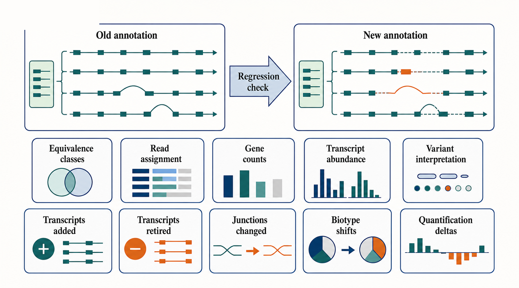
Figure 141.6. Regression checks after annotation updates. Updating a transcript annotation can change equivalence classes, read assignment, gene counts, transcript abundance, and variant interpretation. Regression checks compare old and new releases to identify major coordinate, biotype, and quantification effects.
Recent Consensus
Current transcriptome informatics treats transcript models as evidence-weighted, versioned inferences rather than absolute molecular catalogs. Short-read RNA-seq remains valuable because depth, replication, and mature statistical models support junction discovery, differential expression, and many event-level splicing analyses. Long-read complementary DNA and direct RNA sequencing add molecule-level connectivity across distant exons, transcript ends, haplotype-informative variants, and some native-RNA features, but long reads still require controls for coverage, truncation, internal priming, sequencing error, and alignment artifacts. The consensus position is therefore not that one read class replaces another, but that transcript structure, abundance, termini, allele state, editing state, and reproducibility require different evidence classes that should be interpreted together.
Isoform quantification is now understood as an ambiguity-aware inference problem. Reads compatible with multiple transcripts should not be treated as if they were uniquely assigned molecules unless the evidence actually supports uniqueness. Equivalence classes, transcript compatibility classes, likelihood-based abundance estimation, and uncertainty summaries are central to responsible interpretation. Gene-level aggregation is often more stable than transcript-level quantification, but it can erase biologically meaningful isoform switching, alternative promoter use, alternative polyadenylation, retained-intron regulation, circular RNA isoform structure, and long noncoding RNA isoform balance. Event-level splicing metrics such as percent spliced in are useful when the question is local exon or junction usage; they are not substitutes for transcript-level analysis when coupled events on the same RNA molecule determine the biological outcome.
Annotation updating is also converging on a staged governance model. Discovery workflows can be permissive, but release annotations should be conservative, reproducible, evidence graded, and versioned. Accepted transcript models should distinguish support for structure, abundance, function, reproducibility, and biotype assignment. Rejected or retired models should retain reasons when possible because deprecated transcript models, internal priming artifacts, pseudogene mapping artifacts, and readthrough candidates continue to affect older analyses and future reannotation. Haplotype-aware and RNA-editing-aware transcriptomics are becoming routine enough that annotations and pipelines increasingly need to record when a transcript model, splice choice, or mismatch pattern is allele-specific, edit-specific, population-biased, or reference-dependent.
Open Questions, Controversies, Deprecated Models, and Common Misconceptions
Open questions:
- When should a sample-specific or condition-specific isoform become part of a general reference annotation? Low-abundance lncRNAs, rare disease-associated splice products, cell-state-specific transcripts, circular RNA isoforms, retained-intron RNAs, and transcripts detected in single long-read datasets occupy a gray zone between real biology and release-level annotation. The field lacks universally accepted thresholds for read support, replication, terminal evidence, functional evidence, and cross-sample recurrence. A practical boundary is to separate discovery catalogs from curated releases, but different databases and organism communities still draw that boundary differently.
Controversies:
- Several controversies are interpretation problems rather than simple tool-choice disputes. Event-level splicing analyses can report a significant local change even when the full transcript consequences are uncertain. Transcript-level quantification can report an isoform shift that is conditional on the chosen annotation and may change after annotation updates. Haplotype-aware analyses can reveal allele-specific expression or allele-specific splicing, but they can also amplify reference bias if the reference genome, variant calls, or phasing are incomplete for the sampled population. RNA editing calls are biologically meaningful only after inherited variants, somatic variants, strand errors, read errors, and paralogous mapping artifacts have been considered. These boundary cases are not reasons to avoid the analyses; they are reasons to state the evidence object precisely.
Common misconceptions:
- “A transcript model is identical to a molecule observed in every cell.” Transcript models are annotations; actual molecules vary by cell type, condition, processing state, and evidence support.
- “TPM is an absolute molecule count.” TPM is a relative abundance unit normalized within a sample, not a direct molecule count.
- “PSI is not a full-transcript abundance unless the event definition and transcript structure make that equivalence defensible.” A new annotation release is not automatically more appropriate for an old analysis unless the data are reprocessed and regression checked. A haplotype-specific or editing-specific signal is not a clinical interpretation without sample-matched controls, appropriate validation, and disease-context evidence. The reader-facing rule is simple: state whether the claim concerns assembly, abundance, local splicing, full transcript structure, allele state, editing state, annotation release, or biological function, and then match the evidence standard to that claim.
Deprecated or weakened claims:
- It is obsolete to treat every assembled transcript path as a confirmed RNA molecule, every junction read as proof of a stable isoform, every intron-retention signal as regulated splicing, every RNA-DNA mismatch as editing, or every statistically significant isoform estimate as a functional isoform switch. It is also an overgeneralization to say that long-read data solve isoform quantification by themselves. Long reads improve connectivity, but abundance, rare-isoform detection, sample comparability, and artifact control still depend on library design, depth, replication, and validation.