Chapter 64. RNA Tertiary Modeling, Molecular Simulation, and Machine Learning
Scope Note
This chapter explains how researchers build, simulate, evaluate, and interpret three-dimensional RNA models when direct experimental structures are incomplete, unavailable, or too static for the biological question. The focus is on tertiary modeling rather than secondary-structure prediction alone: base-paired helices, junctions, loops, pseudoknots, tertiary contacts, metal ions, solvent, ligands, proteins, and conformational ensembles must all be considered when an RNA molecule is treated as a physical object in three dimensions.
Executive Summary
RNA tertiary modeling starts from a simple problem statement: a nucleotide sequence and, often, a secondary-structure model are not enough to specify a unique three-dimensional molecule. RNA helices are relatively regular, but the global fold depends on how helices pack through junctions, noncanonical base pairs, base triples, ribose zippers, A-minor interactions, coaxial stacking, pseudoknots, metal-mediated contacts, proteins, small molecules, and environmental conditions. Fragment assembly and homology modeling exploit the empirical fact that many local RNA motifs recur in different contexts. These approaches can be powerful for RNAs built from known motifs, but they fail when the target requires a new topology, an unrecognized ligand-bound state, or a long-range contact that is not encoded in the supplied secondary structure.
Simulation methods ask a complementary question: if an RNA model is treated as a physical system, what motions and alternative conformations are plausible under a chosen potential-energy model? Coarse-grained simulations represent groups of atoms with simplified beads or interaction centers, allowing broader conformational searches and longer timescales. All-atom molecular dynamics represents every atom explicitly and can reveal base-flipping, hydration, ion binding, local rearrangements, and RNA-protein interface dynamics, but it is limited by force-field accuracy, sampling time, and uncertainty in initial structures. Recent reviews of coarse-grained RNA modeling and minimal models emphasize that simplified models are not lesser versions of all-atom models; they answer different questions and make different approximations (Li and Chen 2021; Thirumalai et al. 2025).
The hardest physical problems for RNA simulation are also central to RNA biology. RNA is a highly charged polymer. Its phosphate backbone attracts a diffuse ion atmosphere, and many folded RNAs also contain partially dehydrated or specifically positioned metal ions. Water molecules bridge bases, phosphates, ions, and protein side chains. Force fields must balance base stacking, hydrogen bonding, backbone torsions, sugar puckers, electrostatics, ion coordination, and solvation. Small errors in these terms can make a helix too rigid, a loop too collapsed, a magnesium site too sticky, or a tertiary contact too unstable. A model that looks chemically plausible in a static image may therefore be wrong as a dynamical description.
Machine learning has changed RNA modeling by learning statistical regularities from solved structures, alignments, sequences, and experimental annotations. Geometric deep learning can predict coordinates or inter-residue restraints; transformer and language-model approaches can learn sequence and structure features; and learned scoring functions can rank or refine candidate models. These methods are promising, but the RNA structure database is still much smaller and more biased than the protein structure database. Large ribosomal RNAs, tRNAs, riboswitches, aptamers, and a few recurrent motifs are overrepresented, whereas many cellular noncoding RNAs, transient folding intermediates, modified RNAs, protein-bound states, and ion-dependent conformers remain underrepresented. Reviews of machine learning in RNA structure prediction therefore stress both genuine progress and the need for rigorous benchmarks, uncertainty estimates, and experimental validation (Yu et al. 2022; Zhang et al. 2024; Chaturvedi et al. 2025).
Experimental integration is not an optional afterthought. Cryo-electron microscopy, crystallography, nuclear magnetic resonance spectroscopy, small-angle scattering, chemical probing, crosslinking, mutational profiling, comparative covariation, and biochemical perturbations each constrain different aspects of a model. These data can prune impossible folds, guide sampling, validate predicted contacts, or reveal multiple states. They can also mislead when interpreted as direct geometry: a SHAPE-reactive nucleotide is not simply “unpaired,” a crosslink is not an exact distance, a low-resolution cryo-EM density does not determine every phosphate position, and an evolutionary covariance signal may reflect a conserved alternative state or protein-mediated constraint rather than one static base pair. The strongest RNA tertiary models state what evidence fixes the fold, what evidence only biases it, and what remains uncertain.
Benchmarking must therefore evaluate both accuracy and calibration. A method that predicts one impressive riboswitch fold but gives no confidence estimate is less useful than a method that tells the user when a domain is well constrained and when the output is speculative. Useful benchmarks separate easy homology cases from hard new-fold cases, prevent leakage between training and test structures, compare against experimental ensembles rather than only one deposited coordinate set when appropriate, and report local as well as global error. RNA tertiary modeling is now a hybrid field: empirical motif reuse, physical simulation, machine learning, and experimental restraints are strongest when used together with explicit uncertainty.
Concept Inventory
- Tertiary structure: the three-dimensional arrangement of an RNA molecule beyond its secondary-structure base pairs. In RNA, tertiary structure includes helix orientation, loop-loop contacts, long-range base triples, pseudoknots, metal-binding sites, ligand pockets, protein contacts, and conformational states. A secondary structure can be identical for two RNAs that adopt different tertiary folds.
- Fragment assembly: a modeling strategy that builds an RNA model from libraries of experimentally observed local motifs, such as hairpin loops, internal loops, junction geometries, and noncanonical base-pair steps. The premise is that many RNA local structures recur because the same sugar-phosphate and base-pairing chemistry constrains them.
- Homology modeling: also called comparative or template-based modeling, builds a target model from a known structure of an evolutionarily or structurally related RNA. The method is strongest when the target and template share conserved secondary structure, conserved tertiary motifs, and similar ligand or protein context.
- Coarse-grained modeling: several atoms as one bead or a small set of interaction centers. A nucleotide may be represented by beads for phosphate, sugar, and base, or by an even simpler scheme. Coarse-graining reduces computational cost and smooths the energy landscape, but it removes atom-level information.
- All-atom molecular dynamics: simulates the motion of every atom in RNA, solvent, ions, ligands, and proteins under a force field. The simulation integrates Newtonian equations of motion, usually over femtosecond time steps, to generate a trajectory of conformations.
- Force field: a mathematical energy model describing bonds, angles, torsions, electrostatics, van der Waals contacts, and sometimes specialized terms such as base stacking or ion coordination. A force field is not the true physical energy function; it is a calibrated approximation.
- Ion atmosphere: the ensemble of mobile ions enriched around the negatively charged RNA backbone. It differs from a specifically bound ion site, where an ion occupies a localized structural position with defined coordination geometry or strong functional importance.
- Restraint: an added modeling term derived from information outside the force field, such as a base-pair probability, chemical-probing signal, crosslink, cryo-EM density, NMR nuclear Overhauser effect, or predicted residue-residue distance. A restraint biases model generation; it should not be treated automatically as direct proof.
- Uncertainty: the degree to which a model’s coordinates, contacts, or state assignment are not fixed by the available evidence. Uncertainty can arise from poor sampling, limited training data, ambiguous experiments, real biological heterogeneity, or a wrong modeling assumption.
What to Know Before Reading This Chapter
Readers should be comfortable with RNA polarity, base pairing, stacking, secondary structure, and the distinction between a single structure and an ensemble. Chapter 3 explains why folding depends on free energy and kinetic accessibility rather than only on the minimum-energy state. Chapter 4 introduces the structural motifs that make RNA tertiary folding modular but not fully predictable from sequence. Chapter 61 covers computational secondary-structure prediction, which often supplies the starting helices for the methods discussed here. Chapter 62 and Chapter 63 explain comparative and probing constraints that are frequently converted into tertiary-modeling restraints.
The running examples in this chapter are tRNA, group I introns, riboswitch aptamers, ribosomal RNA domains, and engineered RNA nanostructures. tRNA illustrates a compact, conserved fold with recurrent tertiary interactions. Group I introns illustrate metal-dependent ribozyme architecture and long-range packing. Riboswitch aptamers illustrate ligand-stabilized conformations that may not be apparent from apo-state sequence analysis. Ribosomal RNA illustrates huge assemblies where cryo-EM density, protein contacts, and evolutionary conservation dominate modeling. RNA origami and nanostructures illustrate design-oriented simulation, where the goal is not merely to explain a natural molecule but to predict whether an engineered object will form as intended (Poppleton et al. 2023).
64.1. Fragment assembly and homology-based 3D modeling
Fragment assembly begins with an observation that is easy to underestimate: RNA is chemically flexible, but not infinitely flexible. The ribose-phosphate backbone has allowed torsion-angle combinations, bases prefer stacking and hydrogen-bonding geometries, and many noncanonical base pairs recur. For this reason, the local geometry of a GNRA tetraloop, a kink-turn, an A-minor contact, an E-loop-like motif, or a two-way junction can often be reused in a new molecule when the sequence and pairing context are compatible. Fragment-assembly methods use libraries of such local structures to construct a larger model, then score the model for steric plausibility, base-pair satisfaction, stacking, compactness, and agreement with known or predicted constraints.
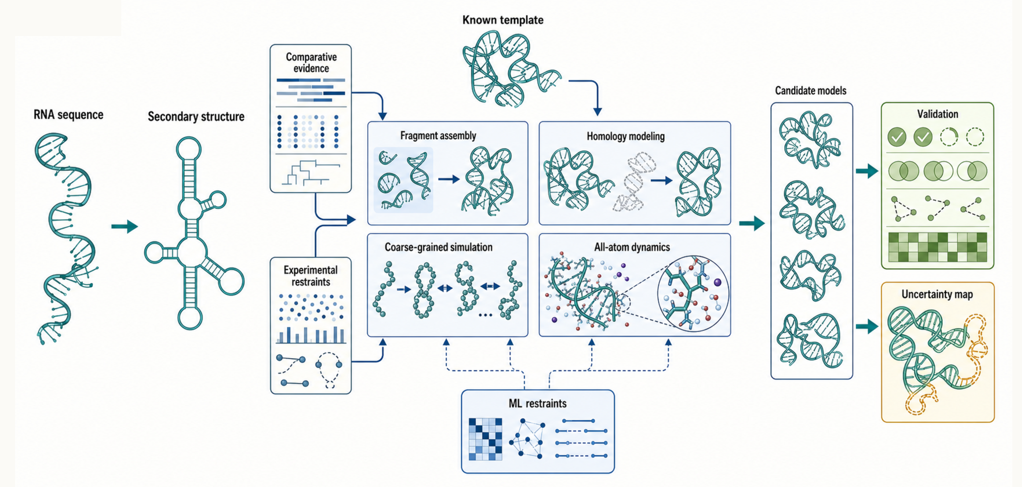
Figure 64.1. Choosing a Modeling Strategy for RNA Tertiary Structure. Starting from an RNA sequence, a modeler usually adds secondary-structure information, comparative evidence, experimental restraints, or known templates before selecting a tertiary-modeling strategy. Fragment assembly is useful when local motifs are known but the global fold must be built. Homology modeling is strongest when a related solved structure exists in the same state. Coarse-grained simulation explores global architecture and conformational alternatives. All-atom molecular dynamics tests local stability, hydration, ion hypotheses, and interface dynamics. Machine-learning restraints can inform any stage, but predictions require calibration and independent validation.
Table 64.1. RNA Tertiary Modeling Methods Compared. RNA tertiary-modeling approaches differ in what information they require, what resolution they can claim, and how their outputs should be validated.
| Method class | Typical input | Typical output | Effective resolution | Strengths | Common failure modes | Best validation data |
|---|---|---|---|---|---|---|
| Fragment assembly | Sequence, secondary structure, motif library | Ranked 3D coordinate models | ~1–3 Å local; lower global | Known-motif and modular RNAs | Unknown topologies, new motifs, library bias | Crystallography, cryo-EM, SHAPE |
| Homology modeling | Sequence, related template structure | Template-derived 3D model | Near-template quality | Conserved-fold RNAs, tRNA, rRNA domains | State mismatch, insertions, non-conserved loops | Independent structural or probing data |
| Coarse-grained simulation | Sequence, secondary structure, coarse-grained potential | Conformational ensemble, folding pathway | Domain-level topology | Folding pathways, large assemblies, nanostructures | Atom-level detail, hydration, catalytic-site chemistry | SAXS, cryo-EM envelope, compaction assays |
| All-atom molecular dynamics | Atomic coordinates, force field, solvent, ions | Time-ordered conformational trajectory | Atomic | Local dynamics, ion binding, interface behavior | Force-field bias, sampling limits, timescale | NMR restraints, crystal contacts, mutagenesis |
| Machine-learning coordinate prediction | Sequence ± secondary structure | Predicted 3D coordinates | Variable | Fast, scalable, captures database patterns | Out-of-distribution RNAs, overconfidence, state conflation | Held-out experimental structures |
| Machine-learning restraint prediction | Sequence, alignment, structure database | Predicted inter-residue distances or contacts | Contact-level | Modular, combinable with physics-based methods | Wrong restraints propagate topology errors | Orthogonal experimental data |
| Integrative experimental modeling | Cryo-EM, NMR, SHAPE, SAXS, covariation | Restrained ensemble or refined model | Data-dependent | Multimodal, grounded directly in experiment | Restraint overinterpretation, state averaging | Orthogonal validation experiments |
Table 64.2. Sources of Uncertainty in RNA 3D Models. Uncertainty in RNA tertiary modeling is regional and context-dependent; a model can be reliable in a conserved helical core while remaining speculative in a peripheral loop, ligand pocket, or ion site.
| Uncertainty source | Example | Affected model feature | Diagnostic control | Reporting recommendation |
|---|---|---|---|---|
| Secondary-structure ambiguity | Alternative base-pair patterns at a junction | Helix orientation, global topology | Test alternative structures; compare constraint satisfaction | Report all alternative folds considered |
| Homology/template mismatch | Template in ligand-bound state, target is apo | Pocket geometry, flexible regions | Align multiple templates; check functional state | State template-state mismatch explicitly |
| Force-field bias | Overstabilized magnesium contact in MD | Ion-site geometry, local stability | Compare replicate trajectories; vary ion parameters | Flag force-field-sensitive contacts |
| Ion-condition uncertainty | Simulation at 150 mM NaCl vs. cellular Mg²⁺ | Compaction, electrostatic shielding, specific sites | Test multiple salt conditions; compare with SAXS | Report ion conditions; distinguish diffuse vs. specific binding |
| Sparse experimental restraints | Few SHAPE-reactive nucleotides constrain a loop | Loop conformation, junction angle | Generate ensemble; measure conformational spread | Indicate underdetermined regions explicitly |
| Cryo-EM local flexibility | Flexible peripheral domain of ribosomal RNA | Peripheral loop, linker position | Multibody refinement; local-resolution estimation | Report local resolution; avoid overfitting atomic models |
| Chemical-probing overinterpretation | SHAPE reactivity interpreted as direct unpairing | Base-pair assignments, secondary structure | Cross-validate with covariation or NMR | Distinguish what probing measures from what it implies |
| ML out-of-distribution prediction | Novel RNA fold absent from training set | Global topology, junction geometry | Compare with template-based or physics-based output | Assess training-data coverage; report confidence per region |
| Training/test leakage | Close homolog of benchmark target in training set | Apparent accuracy inflated | Perform family-level train-test split | Separate interpolation from new-fold benchmarks |
The causal logic is sequential. First, the modeler defines the target RNA sequence and usually an approximate secondary structure. Second, the method decomposes the target into helices, loops, junctions, bulges, and long-range contact candidates. Third, local fragments from solved structures are matched to those elements by sequence, base-pairing pattern, length, motif class, or geometric compatibility. Fourth, the fragments are assembled into candidate global topologies by rotating, translating, and connecting them while preserving chain continuity. Fifth, the candidate structures are filtered and refined to remove steric clashes, broken bonds, impossible backbone geometries, and unsupported tertiary contacts. Finally, candidate models are ranked by a scoring function and, ideally, by independent experimental evidence.
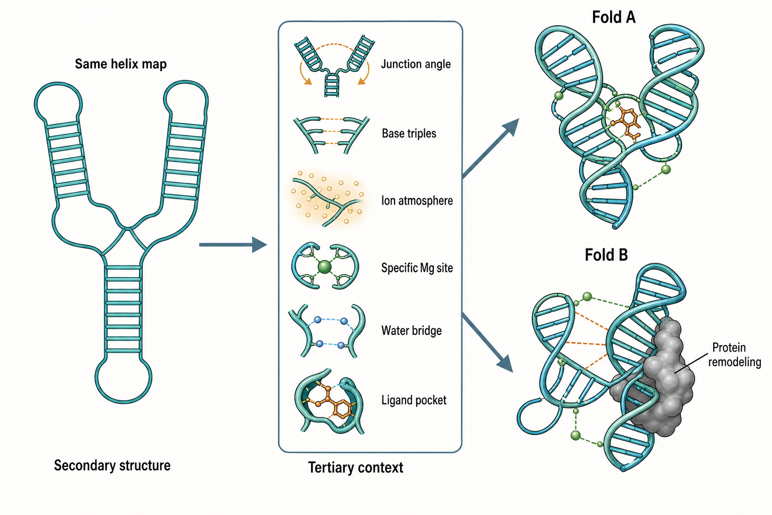
Figure 64.2. Why RNA Tertiary Modeling Is Not Just Secondary Structure in 3D. Two RNAs with the same helix layout in a secondary-structure diagram can differ in tertiary structure because junctions set helix orientation, noncanonical base pairs and base triples make long-range contacts, ions screen or bridge phosphates, water mediates interactions, ligands stabilize pockets, and proteins remodel conformations. A diffuse ion atmosphere and specific metal-binding sites are physically distinct and should be interpreted separately when evaluating any tertiary model.
This workflow is useful because RNA tertiary folds often combine conserved modules in new arrangements. A bacterial riboswitch aptamer, for example, may use standard A-form helices, a junction that organizes helix orientation, a ligand pocket made from noncanonical base pairs, and one or more peripheral contacts that stabilize the ligand-bound conformation. If close homologous structures exist, a model can often capture the main helix arrangement and pocket architecture. If only local motifs are known, fragment assembly may still produce plausible folds, but the global arrangement becomes less certain.
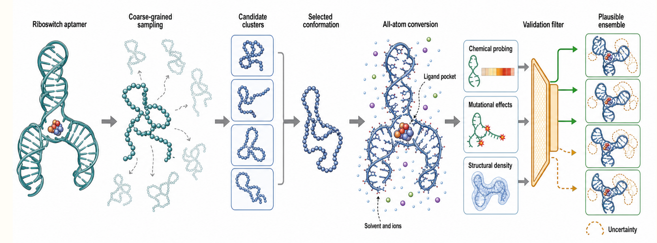
Figure 64.3. Multiresolution Simulation of a Riboswitch Aptamer. A coarse-grained model samples helix packing and ligand-pocket closure across many candidate conformations. A selected candidate is converted to all-atom representation with explicit solvent and ions. Experimental data such as ligand-dependent chemical probing, mutational effects, or structural density are then used to validate which conformational cluster is biologically plausible. The output is an uncertainty-annotated ensemble rather than a single unconditional structure, illustrating how coarse-grained, all-atom, and experimental approaches can be combined for a single RNA target.
Homology-based modeling is more constrained than general fragment assembly. A homologous RNA template is a solved structure from a related RNA family or a structurally similar domain. The method aligns the target sequence to the template, preserves conserved base pairs and tertiary motifs, modifies loops and insertions, and refines regions that differ between target and template. Homology modeling works especially well for RNAs whose fold is more conserved than their sequence, such as many tRNAs, ribosomal RNA domains, and ribozyme cores. It is weaker when the alignment is ambiguous, when insertions create new junction topologies, when a ligand or protein changes the conformation, or when the template represents a different functional state.
The evidence basis for these approaches is the accumulation of RNA structures from crystallography, nuclear magnetic resonance spectroscopy, and cryo-electron microscopy, together with comparative evidence showing that many motifs are conserved by compensatory mutations. Reviews of RNA 3D structure prediction describe fragment reuse and template-based modeling as persistent foundations even as machine learning methods become more prominent (Ou et al. 2022; Wang et al. 2023; Zhang et al. 2024). A structure database is not a neutral sample of all possible RNA folds, however. Ribosomal RNA, tRNA, aptamers, engineered RNAs, and crystallizable domains are overrepresented. Flexible cellular RNAs, transient folding intermediates, heavily modified RNAs, and protein-dependent conformers are less well sampled.
Several boundary cases matter. First, the same secondary structure can support alternative tertiary states. A riboswitch aptamer may have an apo ensemble and a ligand-bound state; a template for one state may mislead modeling of the other. Second, a local motif can recur but change its global role. A kink-turn may be stabilized by protein binding in one RNA and by tertiary packing in another. Third, homologous RNAs can conserve function while changing peripheral architecture. Fourth, fragment assembly tends to prefer familiar motifs; a correct but rare motif may be penalized because the library and score are biased toward known structures.
For this reason, fragment and homology models should be read as hypotheses with domains of reliability. Helical stems and conserved core motifs may be high confidence, whereas peripheral loops, ion sites, flexible linkers, and alternative states may be provisional. Chapter 62 explains how covariance can support conserved pairings and tertiary contacts, and Chapter 63 explains how chemical probing can help distinguish whether a proposed contact is compatible with solution behavior.
64.2. Coarse-grained and all-atom simulations
Molecular simulation asks how a model moves, relaxes, and samples alternative conformations under a specified physical approximation. A static RNA model is a coordinate set. A simulation trajectory is a time-ordered series of coordinate sets generated by a model of forces and thermal motion. This distinction matters because many RNA functions depend on motion: bases flip, helices breathe, junctions switch stacking partners, riboswitch pockets preorganize or close around ligands, and RNA-protein interfaces adapt after binding.
Coarse-grained simulations simplify the molecule so larger systems and longer timescales can be explored. Instead of representing every atom, a coarse-grained model may represent each nucleotide by three beads, one bead, or a small rigid body. The interactions are designed to capture important features such as chain connectivity, excluded volume, base stacking, hydrogen bonding, electrostatics, and sometimes specific tertiary motifs. Because the number of particles is reduced and the energy landscape is smoothed, coarse-grained simulations can sample folding pathways, helix packing, nanostructure assembly, and large conformational rearrangements that would be difficult in all-atom simulations. Li and Chen (2021) review RNA 3D prediction using coarse-grained models, and Thirumalai et al. (2025) emphasize the conceptual value of minimal RNA models for identifying which physical ingredients are essential.
The price of coarse-graining is loss of detail. A three-bead nucleotide model may identify that two helices pack and that a junction bends, but it cannot reliably specify every water-mediated hydrogen bond or magnesium coordination shell. A coarse-grained model may fold a riboswitch into a compact ligand-competent state, but an all-atom or experimentally restrained model may be needed to evaluate whether a small molecule can fit the pocket with correct base-edge contacts. Coarse-grained results should therefore be interpreted at the resolution of the model: topology, relative domain motion, approximate compactness, and likely contact patterns are more appropriate than atom-specific claims.
All-atom molecular dynamics uses a force field to propagate the positions and velocities of atoms in RNA, water, ions, proteins, ligands, and sometimes membranes or other cofactors. The method can reveal local relaxation after model building, identify unstable contacts, compare alternative ion placements, examine RNA-protein interface dynamics, or refine ambiguous experimental structures. For example, all-atom simulations of protein-RNA interfaces can show whether arginine-rich patches remain associated with the phosphate backbone, whether a base-specific contact is persistent, and whether water or ions mediate an apparent interaction (Sabei et al. 2024). All-atom simulation has also been used for ensemble refinement of cryo-EM RNA structures, where a deposited model may contain local geometry errors or overfit one conformation in a heterogeneous density (Posani et al. 2025).
The causal workflow for all-atom simulation begins with an initial coordinate model. The system is assigned protonation states, modified nucleotide parameters if needed, ions, solvent, and boundary conditions. Energy minimization relaxes severe clashes. Equilibration allows solvent and ions to adjust while restraints may hold the RNA near the starting structure. Production simulation then samples molecular motion. Analysts measure root-mean-square deviation, base-pair occupancy, torsion distributions, ion residence, hydrogen-bond lifetimes, stacking, distances, principal components, or transition events. Enhanced-sampling methods, such as replica exchange or metadynamics, add strategies for crossing barriers that would be rare in ordinary simulations.
The key evidence limitation is sampling. A simulation of hundreds of nanoseconds or a few microseconds may be long by computational standards but short relative to RNA folding, ligand binding, or large domain rearrangement. If a contact breaks during simulation, the contact may be physically unstable, the force field may be wrong, the ion conditions may be wrong, or the simulation may have started from an incompatible state. If a contact remains stable, the contact may be real, but it may also be trapped by insufficient sampling. Simulation supports mechanistic interpretation when it is paired with sensitivity analysis, replicate trajectories, appropriate controls, and independent experiments.
RNA nanotechnology provides a useful boundary case. Engineered RNA origami and RNA nanostructures are designed to form target geometries by programmed base pairing and junction architecture. Coarse-grained simulation can screen whether the designed object is geometrically plausible and whether strands or domains assemble without severe strain; all-atom refinement can inspect local motifs, modified residues, or ligand-binding details. Poppleton et al. (2023) review how design, simulation, and application are linked in RNA origami. The same principle applies to natural RNAs: choose the resolution of simulation to match the biological question.
64.3. Ion, solvent, and force-field challenges
RNA modeling is difficult partly because RNA is a polyanion. Every phosphodiester linkage contributes negative charge, so an RNA molecule in solution is surrounded by counterions and water. Some ions form a diffuse ion atmosphere that screens electrostatic repulsion without occupying one fixed site. Other ions bind more specifically, sometimes with inner-sphere coordination in which the ion directly contacts RNA atoms after partial dehydration, or outer-sphere coordination in which water molecules remain between the ion and RNA. Magnesium ions are especially important for many ribozymes and compact RNAs, but potassium, sodium, calcium, polyamines, and proteins can also stabilize RNA architecture.
This physical setting creates a modeling problem at multiple scales. At the global scale, the model must allow negatively charged helices to approach without unrealistic repulsion or artificial collapse. At the local scale, the model must represent hydrogen bonding, base stacking, ribose pucker, backbone torsions, ion coordination, and hydration. At the chemical scale, modified nucleotides, protonated bases, ligands, and catalytic metal sites may require parameters that are not included in standard force fields. A model that treats magnesium as a simple charged sphere may capture screening but not the geometry and kinetics of a catalytic ion site. A model that includes explicit water may reveal bridges that are invisible in a dry schematic, but it also increases computational cost and introduces dependence on water and ion parameters.
A force field divides molecular energy into terms that can be computed efficiently: bond stretching, angle bending, torsional rotation, electrostatics, and van der Waals interactions are common components. For RNA, the balance among these terms is delicate. If base stacking is too favorable, single-stranded regions may collapse into overly stacked conformations. If phosphate repulsion is too strong, tertiary packing may unfold. If torsion parameters favor the wrong backbone rotamers, loops may adopt unrealistic geometry. If ion parameters make magnesium too sticky, simulations may produce long-lived ion bridges that are artifacts. Conversely, if ion binding is too weak, a real ribozyme core may appear unstable.
Force-field challenges are not merely technical details. They affect biological conclusions. Suppose an all-atom simulation of a group I intron active site loses a metal ion needed for catalysis. One interpretation is that the deposited structure captured a crystallization condition that is not stable in solution. Another interpretation is that the simulation lacks the correct ion concentration, protonation state, catalytic substrate, protein cofactor, or force-field balance. A careful study compares conditions, tests alternative ion placements, monitors coordination geometry, and asks whether biochemical data support the simulated state.
Solvent is equally important. Water molecules can bridge bases, stabilize grooves, complete metal coordination shells, and mediate RNA-protein contacts. Cryo-EM and crystallography may not resolve all waters, especially at modest resolution, but simulations require a solvent model. Explicit-solvent simulations represent many water molecules and can capture local hydration patterns, but they are expensive. Implicit-solvent models approximate solvent effects with continuum terms and can accelerate sampling, but they may miss specific water-mediated interactions. Coarse-grained models often treat solvent indirectly, which is appropriate for some folding questions but inadequate for detailed active-site chemistry.
The reference file for this chapter contains fewer directly targeted ion and force-field sources than the topic deserves. The discussion above is therefore supported as a consensus synthesis from the directly relevant RNA modeling and simulation reviews already cited, with final reference item notes needed for specialized reviews on RNA force fields, ion atmosphere theory, and magnesium modeling. Final bibliography item: add verified citations for current RNA force-field benchmarks, magnesium ion parameter evaluations, and ion-atmosphere reviews before final claim-level locking.
Boundary cases include structured RNAs whose ion dependence is indirect. Some RNAs require divalent cations mainly because divalent cations screen charge and favor compaction. Other RNAs require a specific metal ion at a catalytic or ligand-binding site. Still others fold in vivo with protein cofactors and molecular crowding that reduce the apparent need for high magnesium in vitro. A simulation performed at one salt condition should not be generalized automatically to the cell, to a crystallization buffer, or to a therapeutic formulation. Chapter 4 provides the structural principles of ion-stabilized folding, and Chapter 101 should be consulted for how structural methods observe or miss ions and waters.
64.4. ML-based tertiary prediction and restraints
Machine learning in RNA tertiary modeling refers to computational methods that learn relationships among sequence, secondary structure, evolutionary information, experimental annotations, and three-dimensional geometry from data. The phrase covers several distinct tasks. One model may predict base pairs or pseudoknots. Another may predict distances, orientations, torsion angles, solvent accessibility, or contact probabilities. Another may generate full atomic coordinates. Another may score candidate structures or decide which experimental restraints are likely to be reliable. These tasks should not be merged into one vague claim that “machine learning predicts RNA structure.”
Deep learning has been successful in part because RNA structure is geometric. A nucleotide has a position, orientation, base identity, sugar pucker, backbone path, and interaction neighborhood. Geometric deep learning represents molecules as graphs or spatial objects so that predictions respect rotations, translations, and local connectivity. Townshend et al. (2021) introduced a prominent geometric deep-learning approach for RNA structure, and later reviews summarize how graph neural networks, transformers, and language models have expanded the RNA structure toolkit (Yu et al. 2022; Zhang et al. 2024; Chaturvedi et al. 2025). Large language modeling and deep learning have also been applied directly to RNA structure prediction in recent Nature Methods work listed in this chapter’s reference file, although the file lacks verified author names for that entry and should be repaired before final citation use.
Machine-learning restraints are often more useful than end-to-end coordinate predictions. A model can predict that nucleotide i is likely to be close to nucleotide j, that two bases may form a noncanonical pair, that a helix may stack coaxially with another helix, or that a loop resembles a known motif. These predictions can be converted into restraints during fragment assembly, coarse-grained simulation, or all-atom refinement. The advantage is modularity: a learned model supplies statistical information, while physical or geometric modeling enforces chain continuity and chemical plausibility. The risk is that a confident but wrong learned restraint can force the model into an incorrect topology.
Training data are the central constraint. Protein structure prediction benefited from a very large and diverse structure database; RNA has a smaller and more biased archive. Many structures are fragments, engineered constructs, ribosomal components, ligand-bound aptamers, or RNAs solved under nonphysiological conditions. Some RNAs contain modified nucleotides that are missing or simplified in training representations. Many deposited structures are not independent because homologous families appear multiple times. If a training set contains close relatives of a benchmark target, a method may appear to solve de novo prediction while actually performing a form of template recognition. Reviews of machine learning in RNA structure prediction therefore emphasize careful train-test separation and the difference between family-level interpolation and new-fold generalization (Zhang et al. 2024; Chaturvedi et al. 2025).
Machine learning is also used for RNA-small molecule interaction modeling. These models may predict ligand-binding pockets, RNA-binding chemical space, or compound-RNA affinity. The connection to tertiary modeling is direct: a ligand often stabilizes a particular RNA conformation, and a predicted apo RNA structure may not contain the binding pocket observed in the ligand-bound state. Reviews of RNA-targeted small-molecule discovery and machine-learning approaches stress that structure prediction, pocket prediction, chemical representation, and experimental binding data must be integrated carefully (Xiao et al. 2023; Sun et al. 2025). Yazdani et al. (2023) provide an example of machine learning used to characterize RNA-binding chemical space.
The most important boundary case is conformational multiplicity. An RNA may have no single correct structure under all conditions. Riboswitches shift with ligand, temperature, transcriptional timing, and magnesium. Viral RNA elements may adopt alternative long-range contacts during replication, translation, or packaging. Guide RNAs may be structured alone but reorganized inside protein complexes. If a machine-learning model is trained on single deposited structures, it may learn to output one representative state even when the biological reality is an ensemble. A useful prediction should therefore specify state, context, and confidence.
Machine learning should not be treated as a replacement for physical chemistry. A neural model may learn that certain distances or motifs are common, but it does not automatically know whether a new ion condition, modified nucleotide, covalent ligand, or protein interface changes the folding landscape unless such cases are represented in the data or encoded in the architecture. Conversely, physical simulation alone may not sample the right topology without learned or experimental guidance. The emerging consensus is hybrid: machine learning proposes or scores hypotheses, and physics plus experiments test whether the hypotheses are chemically and biologically plausible.
64.5. Experimental integration and validation
Experimental integration means using data from wet-laboratory or structural methods to build, restrain, select, or validate RNA tertiary models. Validation means testing whether a model explains data that were not simply used to force the model. These two operations should be distinguished. A cryo-EM density map used to build a ribosomal RNA model cannot also serve as fully independent proof that every local contact is correct. A chemical-probing profile used as a restraint cannot independently validate the same constrained base-pair pattern. Strong validation uses orthogonal evidence.
High-resolution structural methods provide the most direct coordinate information. X-ray crystallography can yield detailed atomic models when crystals diffract well, but crystallization can select one conformation, introduce lattice contacts, require truncations, or use buffer conditions different from the cellular context. Nuclear magnetic resonance spectroscopy can provide local distance and torsion restraints and can reveal dynamics for smaller RNAs, but size, spectral overlap, and conformational heterogeneity limit many systems. Cryo-electron microscopy can resolve large RNA-protein assemblies and multiple conformational classes, but local RNA geometry may be uncertain in flexible regions or at modest resolution. Modelers must therefore ask which parts of the structure are experimentally determined and which parts are fitted, idealized, or inferred.
Low-resolution and ensemble-sensitive methods provide complementary constraints. Small-angle X-ray scattering reports approximate size and shape in solution. Chemical probing methods such as selective 2′-hydroxyl acylation analyzed by primer extension and dimethyl sulfate probing report nucleotide reactivity that correlates with local flexibility, pairing, stacking, or accessibility, but reactivity is not a direct 3D coordinate. Crosslinking can indicate proximity, but crosslink formation depends on chemistry, orientation, light exposure, and accessibility. Mutational profiling can identify nucleotides important for structure or function, but a deleterious mutation may disrupt folding, ligand binding, transcription, processing, or stability indirectly.
The causal integration workflow is similar across data types. First, define what the experiment measures physically. Second, convert that measurement into a restraint or likelihood term with an uncertainty model. Third, generate an ensemble of structures rather than one forced model when the data are sparse. Fourth, hold out some data or use independent data for validation. Fifth, report which regions are well constrained and which remain underdetermined. Chapter 63 covers probing-constrained modeling in more depth; this chapter emphasizes that probing data become more powerful when combined with tertiary-aware modeling and less reliable when interpreted as a direct structure readout.
A riboswitch aptamer illustrates experimental integration well. A secondary-structure model may identify conserved helices. Covariation may support some base pairs. A ligand-bound crystal or cryo-EM structure may show the binding pocket. SHAPE or DMS data may indicate which nucleotides become protected upon ligand addition. Mutations in the pocket may alter ligand affinity. A molecular simulation may test whether the pocket remains stable without crystallographic contacts. A strong model explains these observations together: conserved nucleotides form the pocket, ligand addition stabilizes a specific tertiary arrangement, reactivity changes occur near flexible-to-ordered regions, and mutations disrupt contacts predicted by the structure. A weak model merely fits one data type while ignoring contradictions.
RNA-protein complexes add another layer. A guide RNA inside a CRISPR effector, a spliceosomal snRNA, or a ribosomal RNA segment may adopt a protein-stabilized conformation that is not favored by the naked RNA. Modeling the RNA alone can be useful for identifying intrinsic motifs, but validation must consider the complex. All-atom simulations of protein-RNA interfaces and cryo-EM ensemble refinement are examples of computational approaches that explicitly address the coupled system rather than treating RNA as isolated (Sabei et al. 2024; Posani et al. 2025).
Experimental artifacts must be named close to the relevant claim. Chemical probing can be affected by reverse-transcription stops, RNA abundance, modification status, protein protection, and reagent accessibility. Cryo-EM maps can average multiple conformations or lose flexible elements. Crystallography can stabilize non-native contacts. NMR may require constructs that remove peripheral domains. Crosslinking can enrich rare but reactive geometries. None of these limitations makes the methods unreliable by default. They mean that modeling should preserve the distinction between measured signal, interpreted structural feature, and biological mechanism.
Box 64.1. How to Read Confidence in an RNA 3D Model
- Check whether the model is template-based, physics-based, ML-generated, experimentally restrained, or a hybrid; each source has characteristic strengths and failure modes.
- Identify the modeled state: apo, ligand-bound, protein-bound, specific ion condition, construct boundaries, species, and temperature if known.
- Separate high-confidence conserved cores from flexible or weakly restrained peripheral regions; confidence is regional, not a single file-level property.
- Ask whether validation data were independent of the data used during model building; a restraint used for fitting cannot serve as independent proof.
- Treat specific ion sites, ligand poses, and catalytic geometries as high-evidence claims that require structural or biochemical support beyond the model itself.
64.6. Benchmarking and uncertainty
Benchmarking is the practice of evaluating modeling methods on defined test cases with transparent metrics. For RNA tertiary modeling, benchmarking is difficult because the answer is not always one coordinate set. The deposited structure may be one state, one construct, one buffer condition, one ligand state, or one member of a heterogeneous ensemble. A method may correctly predict the conserved core but miss a flexible peripheral loop. Another method may produce a low global root-mean-square deviation because most helices are placed well, while failing at the active site that matters biologically. A benchmark that reports only one global number can hide these differences.
Useful metrics include global root-mean-square deviation, local distance difference measures, interaction-network fidelity, base-pair recovery, noncanonical-pair recovery, clash scores, backbone torsion quality, ligand-pocket accuracy, ion-site accuracy, and agreement with independent experimental data. For some questions, topology is the main metric: are the helices packed in the right order, and are the long-range contacts present? For other questions, atomic detail is essential: does a catalytic guanosine in a ribozyme occupy the right position relative to a metal ion and scissile phosphate? A benchmark should match the metric to the intended use.
Train-test leakage is a major issue for machine learning and template-based modeling. If a target RNA has close homologs or nearly identical motifs in the training set, the method may be evaluated on recognition rather than prediction. This is not necessarily bad; recognizing that a target belongs to a known fold family is valuable. But benchmark reports should separate template-rich cases from genuine extrapolation. Homology-aware benchmarking and family-level splits are therefore essential for judging generalization.
Uncertainty should be reported at multiple levels. Sequence-level uncertainty includes ambiguous alignment, unknown modification status, and uncertain transcript boundaries. Secondary-structure uncertainty includes alternative pairings and pseudoknots. Tertiary uncertainty includes helix orientation, loop placement, ion sites, ligand-bound state, and flexible domains. Method uncertainty includes force-field bias, sampling insufficiency, experimental noise, and training-data bias. A model can be high confidence in one region and low confidence in another. Reporting only a single confidence score encourages overinterpretation.
Ensemble thinking is a practical solution. Instead of asking for one “best” model, researchers can generate a distribution of models consistent with the evidence. If all plausible models share a core contact, that contact is more reliable. If models diverge in one junction, that junction is underdetermined and may be flexible. If two conformational clusters both satisfy the data, the RNA may have alternative states or the data may be insufficient. Ensemble refinement of cryo-EM RNA structures using all-atom simulations exemplifies this shift from one static coordinate set toward uncertainty-aware structural interpretation (Posani et al. 2025).
Benchmarking also needs negative controls. A method should be tested on RNAs outside its intended domain, on shuffled or incompatible restraints, and on cases where the correct answer requires a ligand, protein, ion, or modification absent from the input. Failure modes are scientifically useful. They reveal when a model is using superficial sequence similarity, when a scoring function prefers overpacked structures, when a force field destabilizes native loops, or when a neural network is overconfident on out-of-distribution RNAs.
The reference file for this chapter includes several benchmarking papers from RNA-seq, editing, and single-cell contexts that are not directly about tertiary modeling. They are useful reminders of benchmarking principles but not direct evidence for RNA 3D prediction. Final bibliography item: add verified RNA-Puzzles, CASP/RNA-related, and current RNA 3D prediction benchmark references before finalizing this chapter’s benchmark section. Until then, this section should be treated as consensus synthesis from RNA structure prediction reviews plus general benchmark logic, not as a complete citation map.
Box 64.2. Worked Example: Ligand-Stabilized Riboswitch Modeling
- Begin with the RNA sequence and identify conserved secondary-structure helices from comparative sequence analysis.
- Add covariation-supported tertiary contacts as candidate restraints, noting that each covariance signal may reflect a conserved pairing or a protein-mediated constraint.
- Use a ligand-bound template or fragment assembly to build the aptamer core, recording the functional state assumed at every stage.
- Compare chemical-probing profiles in the apo and ligand-bound states to identify nucleotides that become ordered or protected upon ligand addition.
- Apply coarse-grained and then all-atom simulations to test whether the predicted pocket remains stable and which junction conformations are accessible without crystallographic contacts.
- Validate with point mutations that disrupt predicted pocket contacts and confirm loss of ligand affinity without globally disrupting the fold.
- Report the model as state-specific: the biologically relevant conformation is stabilized by ligand, specific ions, and transcriptional context, and may not represent the apo ensemble.
Recent Consensus
Recent consensus is that no single method solves RNA tertiary modeling across all molecule classes and contexts. Fragment assembly and homology modeling remain strong when the target contains known motifs or belongs to a structurally characterized family. Coarse-grained simulation is valuable for folding pathways, domain organization, and design screening. All-atom simulation is valuable for local dynamics, interface behavior, ion and solvent hypotheses, and refinement, but it is limited by force fields and sampling. Machine learning has improved tertiary prediction and restraint generation, especially through geometric representations and sequence-trained models, but RNA training data remain small, biased, and state-specific compared with protein data (Yu et al. 2022; Zhang et al. 2024; Chaturvedi et al. 2025).
The strongest practice is integrative. A credible model states the starting assumptions, data sources, modeling method, confidence by region, and validation evidence. It distinguishes a conserved core from flexible periphery, a ligand-bound state from an apo ensemble, a diffuse ion atmosphere from a specific metal site, and a fitted restraint from an independent test. For many RNAs, the correct scientific object is not one structure but a conditional ensemble.
Open Questions, Controversies, Deprecated Models, and Common Misconceptions
Open questions:
- How accurately can current force fields represent divalent-ion effects, modified nucleotides, and long-timescale RNA conformational changes in systems larger than small motifs? The field has improved, but specialized ion coordination, catalytic sites, and rare transitions remain hard.
- How far can machine-learning models generalize beyond known RNA families and solved structural classes? Apparent progress can be inflated by homologous test cases, motif recurrence, or benchmark leakage. The useful distinction is not machine learning versus physics, but calibrated prediction versus overconfident extrapolation.
- How should models represent cellular context? Many RNAs fold co-transcriptionally, bind proteins, experience crowding, contain modifications, and occupy compartments. Modeling purified RNA in dilute solution can answer important questions but may not represent the cellular state.
Common misconceptions:
- “A predicted 3D RNA model is equivalent to an experimental structure.” A model is a hypothesis constrained by assumptions, training data, scoring functions, and available evidence. Even experimental structures contain modeled regions and uncertainty.
- “Magnesium dependence means a specific magnesium ion must be placed in the structure.” Many magnesium effects are diffuse electrostatic or ensemble effects. Specific ion sites require stronger evidence, such as resolved density, biochemical metal-rescue logic, or consistent simulation and structural support.
- “Chemical probing directly reports base pairing.” Probing reports chemical reactivity under a condition. Reactivity often correlates with flexibility or exposure, but it can be affected by protein binding, modifications, local chemistry, and reagent access.
- “The lowest-energy or highest-scoring model is necessarily the biological state.” Biological RNAs can be kinetically trapped, ligand-stabilized, protein-remodeled, or functionally dynamic. Energetic ranking must be interpreted with context.