Chapter 124. Quantitative RNA Biochemistry: Binding, Kinetics, Stoichiometry, and Catalysis
Scope Note
This chapter explains how purified RNA, proteins, and ribonucleoprotein complexes are converted into quantitative biochemical measurements. Its primary ownership is measurement physics, experimental design, quantitative models, parameter estimation, and reporting for binding and catalytic assays. It does not replace the biological account of RNA recognition and assembly in 56, the structural and biophysical determination methods in 59, or the mechanistic treatment of particular enzymes and RNP machines in their pathway chapters. Instead, it supplies the common language needed to decide whether a reported affinity, rate constant, stoichiometry, or catalytic parameter is actually identified by the experiment.
Executive Summary
Quantitative RNA biochemistry begins before an instrument produces a signal. An RNA concentration determined from absorbance counts molecules that absorb light; it does not prove that every molecule has the intended length, chemical ends, fold, ligand accessibility, or catalytic competence. Protein concentration likewise does not equal active binding-site concentration. The active fraction is the fraction of nominal material capable of participating in the modeled reaction. If active fraction is ignored, a binding titration can appear weaker, a calorimetric stoichiometry can appear nonintegral, and an enzyme turnover number can be underestimated. Preparation, folding, labeling, concentration measurement, and substrate-competence tests therefore belong to the quantitative model rather than to an informal prelude.
Different assays answer different questions. An equilibrium titration estimates how species are distributed after sufficient time under fixed conditions. A kinetic experiment measures how quickly that distribution changes. A stoichiometric measurement asks how many competent components occupy a complex. A catalytic experiment asks how substrate conversion depends on time and concentration. A single number called a “binding constant” cannot substitute for association and dissociation rates when residence time matters, and an apparent half-saturation concentration is not automatically a thermodynamic dissociation constant. In tight-binding experiments, ligand depletion causes free concentrations to differ from total concentrations. In cooperative, competitive, multistate, or coupled-folding systems, a one-site hyperbola may fit smoothly while representing the wrong physical model.
Solution methods and surface methods impose different perturbations. Electrophoretic mobility shift assays (EMSAs), filter binding, anisotropy, and competition experiments can be economical and sensitive, but labels, separation, filters, and nonequilibrium handling can distort the species distribution. Isothermal titration calorimetry (ITC) reports heat and can jointly inform affinity, enthalpy, and an apparent stoichiometry, provided concentrations, heats of dilution, active fractions, and the information content of the titration are adequate. Surface plasmon resonance (SPR) and biolayer interferometry (BLI) record association and dissociation in real time, but immobilization, mass transport, surface heterogeneity, rebinding, and nonspecific adsorption can make fitted rates properties of the assay geometry rather than of the solution reaction. Microscale thermophoresis (MST) is performed in solution-filled capillaries and uses a fluorescence response to a temperature gradient, yet fluorescence artifacts, adsorption, aggregation, and thermophoretic complexity still require controls.
Catalytic measurements must distinguish steady-state, pre-steady-state, and single-turnover regimes. A Michaelis-Menten fit summarizes a specific experimental regime; its parameters do not necessarily map one-to-one onto binding and chemistry steps. Initial-rate analysis can conceal bursts, lags, substrate inhibition, product inhibition, inactivation, or a slow conformational transition. Pre-steady-state and single-turnover experiments can resolve steps that are averaged together during repeated turnover, but only when mixing dead time, signal calibration, and substrate competence are controlled. Coupled assays add a reporting reaction whose capacity and lag must be shown not to limit the primary RNA-dependent reaction.
Model fitting is an experiment-model comparison, not a ceremonial final step. Parameters are identifiable only when the data constrain them within a useful range. Replicate scatter, confidence intervals, likelihood profiles, posterior distributions, residual structure, and sensitivity to alternative models convey different aspects of uncertainty. Global fitting across concentrations, observables, and perturbations can identify shared parameters that separate fits cannot, but sharing a parameter is a mechanistic assumption that must be justified. The strongest studies combine orthogonal observables, perturb the concentration and time regimes, disclose raw or minimally processed traces, and report enough detail for another laboratory to reproduce both the reaction and the inference.
Concept Inventory
- Nominal concentration: concentration inferred from mass, absorbance, fluorescence, or another bulk measurement without correction for reaction competence.
- Active concentration: concentration of molecules capable of the specific binding or catalytic event represented in the model.
- Equilibrium dissociation constant, K_D: for a defined association such as P + R ⇌ PR, the ratio
[P][R]/[PR]at equilibrium under specified conditions. It is a thermodynamic property of the stated species and conditions, not a universal property of a sequence. - Kinetic rate constant: a parameter describing the time dependence of a defined elementary or lumped step, such as association
k_onor dissociationk_off. - Stoichiometry: the number or ratio of molecular components in a defined complex. Apparent stoichiometry can differ from molecular stoichiometry when active fractions are below one or states are heterogeneous.
- Ligand depletion: a regime in which complex formation appreciably changes the free concentration of a titrated species, invalidating an approximation that free and total concentrations are equal.
- Specific activity: observed activity per nominal amount of sample under specified assay conditions; it is useful for quality comparison but is not itself an intrinsic catalytic constant.
- Steady state: a kinetic regime in which concentrations of enzyme intermediates change slowly relative to flux through the cycle, even though substrate is being converted to product.
- Single turnover: a regime commonly created with active enzyme or RNP in excess over substrate, such that each substrate molecule is converted at most once and product release need not support repeated cycles.
- Global fit: simultaneous fit of multiple datasets to one explicit model with selected parameters shared across datasets.
- Structural identifiability: whether unique parameter values are theoretically recoverable from ideal data for the model and observables.
- Practical identifiability: whether the actual experiment, with its sampling, range, and noise, constrains the parameters.
What to Know Before Reading This Chapter
RNA is a polyanion whose fold and association behavior depend on sequence, temperature, pH, monovalent and divalent ions, counterions, and molecular crowding. A purified RNA can occupy several slowly interconverting structures. RNA-binding proteins can oligomerize, aggregate, lose cofactors, retain copurifying nucleic acid, or contain only a fraction of competent binding sites. These properties make the chemical species in a tube less obvious than their labels suggest. Chapters 2 and 3 provide the chemical and folding background; this chapter asks how those physical states enter quantitative inference.
The running binding example is an RNA-binding protein, Puf4, interacting with a cognate RNA. The simplest model is P + R ⇌ PR, with K_D = k_off/k_on only when the same one-step reversible mechanism and consistent concentration standards describe both equilibrium and kinetic measurements. The running catalytic example is an RNA-processing enzyme or ribozyme that binds substrate S, proceeds through one or more chemical or conformational steps, and forms product P. A helicase ATPase assay supplies a second catalytic example because the measured signal may report ATP consumption while the biological question concerns RNA duplex unwinding.
A measured signal is not a species concentration until a response model connects them. A gel band intensity may be proportional to labeled RNA, anisotropy is a weighted optical property of fluorescent species, SPR response reflects material near a surface, and absorbance in a coupled assay may report a cofactor consumed by a second enzyme. Before interpreting a curve, identify the material entering the experiment, the physical event generating signal, the mapping from signal to species, and the assumptions connecting species to parameters.
124.1. RNA and RNP preparation, folding, concentration, labeling, and active fractions
Define the reacting material
The object called “RNA” in a reaction should be described by sequence, length distribution, terminal chemistry, modification state, counterion history, purification method, and folding protocol. In vitro transcription can leave heterogeneous 5′ or 3′ ends, abortive products, double-stranded contaminants, and triphosphate termini. Chemical synthesis can introduce deletion products or protecting-group remnants. Native RNA can contain modifications and bound factors that a recombinant substrate lacks. Denaturing purification establishes length separation but also erases the starting fold; native purification may preserve an assembly but can retain heterogeneous partners. No single preparation is universally superior. The required characterization follows from the claim.
For an RBP affinity experiment, denaturing polyacrylamide gel electrophoresis can establish a dominant RNA length, and analytical native electrophoresis or size-exclusion behavior can reveal gross aggregation. For a catalytic RNA, endpoint conversion under enzyme excess can estimate the fraction of substrate able to reach product. For a riboswitch, a binding-competent fraction can be compared across refolding conditions by a saturating-ligand titration. These tests do not prove a unique fold, but they constrain whether the nominal substrate population matches the modeled population.
RNA folding protocols are interventions. Heating, snap cooling, slow cooling, and staged addition of magnesium can populate different states. The solution should reach the final buffer and temperature before the clock for equilibration begins. A protocol that dilutes a folded RNA into a new ionic environment may initiate refolding during the assay. If the transition is slow, two samples with identical final composition can produce different results because their histories differ. Report order of addition, incubation time, temperature, buffer species, ionic strength, free divalent-ion concentration when known, reducing agents, carrier or detergent additives, and any crowding agent.
Proteins and RNPs require parallel scrutiny. Purity by stained gel is not equivalent to monodispersity or activity. Copurifying nucleic acid can be detected by absorbance ratios, nuclease sensitivity, or mass/size analysis. Oligomerization can change with concentration and salt. Freeze-thaw cycles, proteolysis, oxidation, missing metal, and substoichiometric cofactors can reduce competence. An RNP assembled from separately measured components may have an assembly yield below one even when each component is individually pure. Biological ownership of the assembly mechanism remains in 56; the quantitative point here is that the concentration assigned to the reacting species must reflect the assembled and competent population.
Concentration is a model input
Ultraviolet absorbance at 260 nm is commonly used for RNA concentration, but the extinction coefficient depends on base composition and hypochromicity, and contaminants or turbidity can bias the reading. Fluorescent dyes can provide sensitivity but respond differently to single-stranded RNA, duplex RNA, structured RNA, and contaminants. Phosphate analysis, quantitative hydrolysis, isotope dilution, amino-acid analysis for proteins, or calibrated elemental methods can provide independent concentration information in demanding cases. Dilution accuracy, adsorption to vessel walls, and evaporation matter when the final amount is picomolar or the sample volume is small.
An uncertainty in concentration propagates systematically into fitted parameters. A twofold error in active protein concentration can move an affinity estimate, apparent stoichiometry, or k_cat even if replicate curves are precise. Technical replicates from the same stock will not reveal the common stock error. Independent preparations, orthogonal concentration measurements, or fitting an active-fraction parameter against a stoichiometric assay can address different parts of this uncertainty.
Labels can change the reaction
Radioisotopes, fluorophores, biotin, affinity tags, spin labels, and surface-coupling groups provide sensitivity or immobilization, but they also alter mass, charge, hydrophobicity, steric accessibility, and sometimes fold. A 5′ fluorophore may be benign for one RNA and disruptive when the 5′ end forms a helix or contacts protein. Biotin-streptavidin attachment can orient a molecule but can also create avidity or steric occlusion. Protein tags can change oligomerization or RNA affinity. The control is not merely that the labeled material gives signal: labeled and unlabeled materials should be compared by competition, activity, mobility, or another independent assay.
Labeling efficiency creates mixtures. If only a fraction of RNA carries fluorophore, the optical signal reports that fraction, whereas bulk concentration reports all RNA. Free dye can produce a large background in anisotropy or MST. Radiochemical decay, photobleaching, quenching, and environment-sensitive fluorescence can make response factors state- and time-dependent. The analysis should specify whether concentration refers to total molecules, labeled molecules, or competent labeled molecules.
Active fraction links preparation to inference
The active fraction can be estimated by stoichiometric titration when a trusted partner is present at a concentration well above the relevant K_D, by active-site titration using a near-irreversible inhibitor or substrate, by endpoint conversion under forcing conditions, or by comparison with a calibrated standard. Each method defines activity relative to a reaction. A protein may be active for RNA binding but inactive for catalysis, and an RNA may bind but fail to undergo the required conformational transition.
Consider a preparation with 100 nM nominal Puf4 but 50% active protein. If 100 nM is used as the free-protein axis, the apparent curve is displaced. In a tight-binding titration the midpoint can primarily report the concentration of competent sites rather than K_D. Conversely, a saturating titration with trace labeled RNA may report the active fraction but provide only an upper bound on a very small K_D. The experiment must be designed to separate concentration and affinity rather than expecting one curve to identify both.
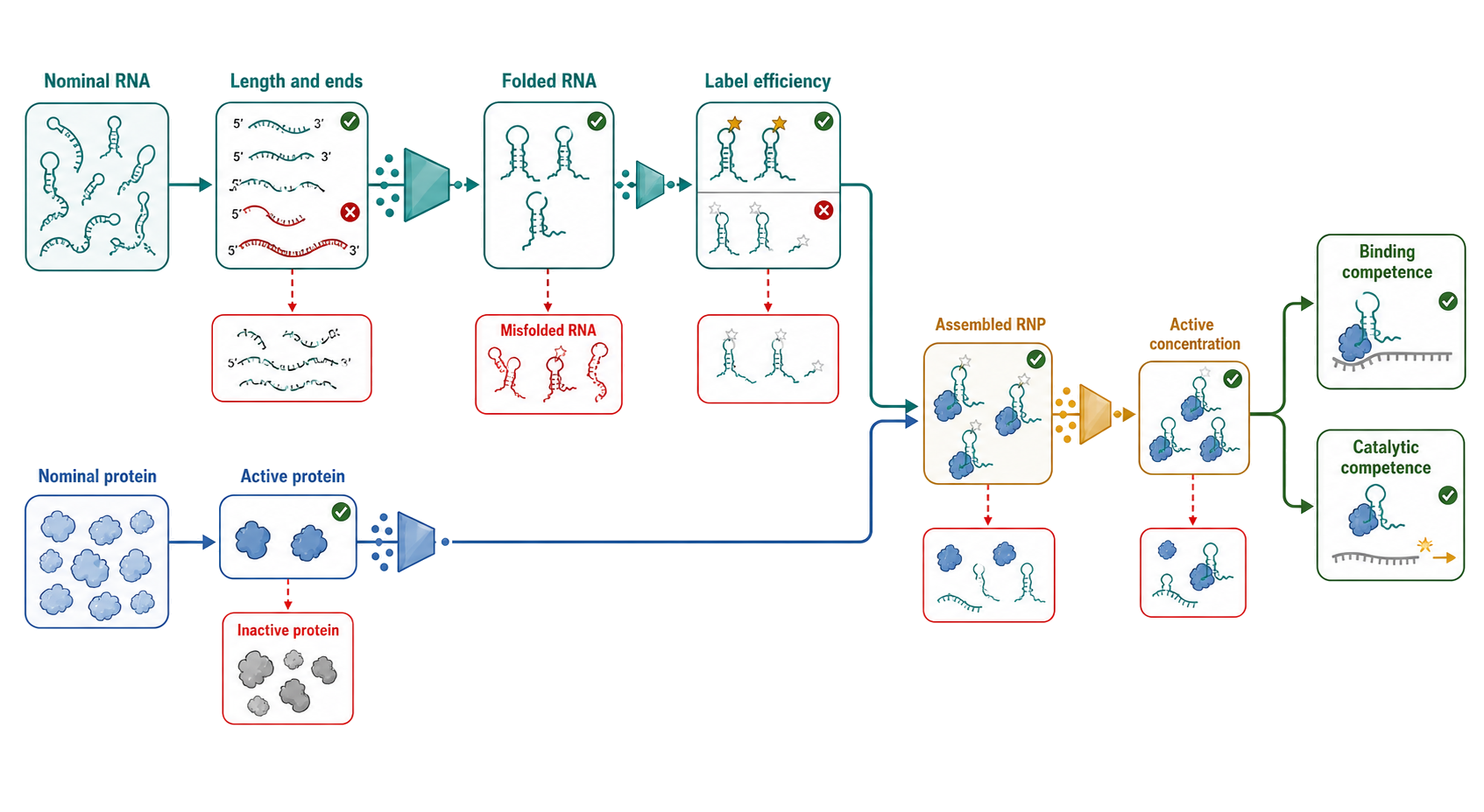
Figure 124.1. Nominal material is filtered into active reacting species. “A bulk concentration enters an assay only after preparation-dependent gates. Active fraction is defined relative to the reaction being modeled.”
Table 124.1. Material-competence checks before quantitative fitting. Connect a preparation risk to a discriminating check and model consequence.
| Risk | Check | If unresolved | Parameter most affected |
|---|---|---|---|
| RNA length or end heterogeneity | Denaturing separation and end-appropriate analysis | Mixed chemical species | Amplitude, stoichiometry, catalytic rate |
| Misfolded RNA | Refolding-history comparison and saturating competence assay | Multiple reactive populations | Active fraction, apparent affinity |
| Inactive protein | Active-site or stoichiometric titration | Nominal concentration exceeds active sites | K_D, n, k_cat |
| Copurifying nucleic acid | Absorbance, nuclease sensitivity, mass/size analysis | Occupied or aggregated protein | Affinity and oligomer state |
| Incomplete labeling | Label-efficiency and free-label measurement | Signal concentration differs from bulk | Fraction bound, anisotropy amplitude |
| RNP assembly below one | Component and assembled-complex assays | Mixed free and assembled material | Stoichiometry and kinetics |
124.2. Equilibrium binding by EMSA, filter binding, anisotropy, fluorescence, and competition
Equilibrium is a condition, not an incubation time chosen by habit
An equilibrium binding experiment holds composition and conditions fixed long enough that forward and reverse fluxes balance. Equilibration should be tested by varying incubation time and, where feasible, by approaching the final state from different starting conditions. A slow dissociation rate can require hours even when association appears rapid. Cooling a reaction can stabilize complexes during gel loading but can also change the equilibrium. If the assay separates bound and free species, the separation step must be fast relative to dissociation or explicitly modeled.
For a simple 1:1 interaction under trace-ligand conditions, fraction bound follows a hyperbola in free protein concentration and the half-saturation point equals K_D. This convenient approximation fails when the labeled RNA concentration is not much lower than K_D. Complex formation then depletes free protein and RNA, and the total concentrations must be related through mass balance, often with a quadratic binding equation. Even a quadratic equation cannot create information that is absent: in a strongly stoichiometric titration the curve can constrain active site concentration while leaving the lower bound of K_D poorly identified.
EMSA and filter binding
An electrophoretic mobility shift assay separates free labeled nucleic acid from complexes that migrate differently through a native gel. EMSA can reveal several mobility classes, distinguish grossly different stoichiometries, and use little material. A fluorescent EMSA or radiometric EMSA can be quantitatively analyzed if signal response is linear and all labeled species are included. However, a gel band is a species operationally stable during loading and electrophoresis. Dissociation in the gel, reassociation, material trapped in wells, conformational mobility shifts, and complexes too heterogeneous to enter the gel can distort the equilibrium distribution.
Filter binding retains one partner or complex on a membrane while another species passes through. Double-filter arrangements can separately capture protein-bound nucleic acid and free nucleic acid. The assay is rapid and suited to many samples, but retention efficiency, filter saturation, nonspecific adsorption, washing-induced dissociation, and loss of aggregates must be measured. Neither EMSA nor filter binding should infer the fraction bound by dividing one selected band or filter signal by an incomplete total.
The Puf4-RNA system illustrates a sound titration. Use trace labeled RNA at several concentrations, titrate active protein over a range spanning below and above the expected transition, establish the equilibration time, and repeat selected points with altered incubation. Quantify all RNA-containing regions. Varying the trace RNA concentration tests for ligand depletion. A nonspecific RNA and a sequence mutant test selectivity, but selectivity is a relative thermodynamic property and should not be confused with absence of all nonspecific binding.
Fluorescence anisotropy and other solution signals
Fluorescence anisotropy reports the polarization retained between excitation and emission. A small fluorescent RNA tumbles rapidly; binding a larger protein often slows rotational diffusion and increases anisotropy. The measurement is homogeneous—no physical separation is required—and can be read over time. Yet anisotropy is not literally fraction bound. It is an intensity-weighted property of fluorescent species and depends on fluorophore lifetime, local motion, quenching, scattering, viscosity, and instrument geometry. A protein-induced change in dye environment can alter intensity and anisotropy without the assumed mass change.
Fluorescence intensity, Förster resonance energy transfer, and environment-sensitive dyes can report association or conformational change. Their strength is temporal resolution and low material use; their weakness is that the signal may conflate binding with structural rearrangement. A response calibration should determine the signal of free and saturated states, and control titrations should test whether protein fluorescence, absorbance, quenching, or aggregation changes the readout. If the saturated signal varies with protein concentration, a two-state linear mixture is inadequate.
Competition reveals solution affinity only through a model
Competition assays are useful when an unlabeled RNA cannot be directly observed, when the direct interaction is too tight for the accessible concentration range, or when relative specificity is the question. A preformed labeled complex is challenged with unlabeled competitor, or both ligands are equilibrated together. The fitted inhibition midpoint depends on labeled-probe concentration, tracer affinity, active receptor concentration, depletion, and competition mechanism. An IC50 is therefore not automatically the competitor K_D.
A valid competitive model states whether ligands exclude one another from one site, bind distinct sites allosterically, or form ternary complexes. It also accounts for competent concentrations. A competitor can appear weak because it folds slowly, aggregates, or binds a nonproductive protein state. Conversely, a contaminant with high affinity can dominate at low nominal abundance. Competition and direct assays are powerful orthogonal partners because they perturb labels and concentration regimes differently.
Cooperative binding requires special care. A sigmoidal curve can arise from genuine energetic coupling, multiple nonidentical sites, ligand depletion, oligomerization, aggregation, or a signal nonlinearity. A Hill coefficient is a descriptive slope, not a direct count of sites and not by itself proof of cooperativity. Mechanistic binding polynomials or explicit state models should be used when the data and independent stoichiometric information justify them.
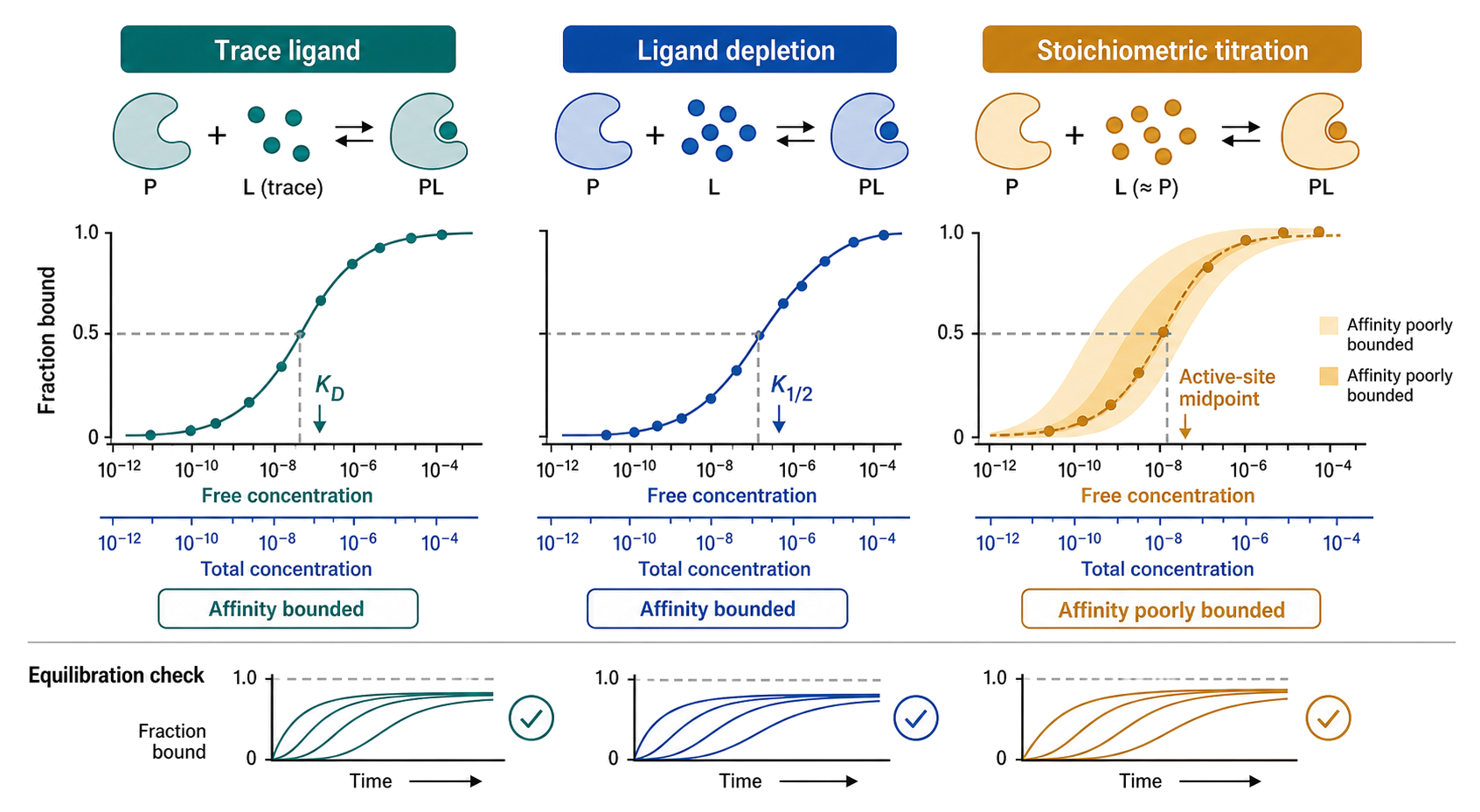
Figure 124.2. Binding, depletion, and stoichiometric titration regimes. “Half-saturation equals K_D only for the stated simple equilibrium and an appropriate concentration regime. Tight titrations often identify active-site concentration more strongly than affinity.”
Table 124.2. Equilibrium binding assays and their physical outputs. Prevent platform output from being mistaken for fraction bound without calibration.
| Assay | Direct observable | Major strength | Dominant artifacts | Essential perturbation |
|---|---|---|---|---|
| EMSA | Mobility distribution of labeled RNA | Resolves operational complex classes | Dissociation, trapping, missing material | Time and gel-condition variation |
| Filter binding | Retention on one or more membranes | Rapid and scalable | Retention efficiency, washing loss | Filter and wash controls |
| Fluorescence anisotropy | Polarization-weighted fluorescence | Homogeneous solution readout | Dye motion, intensity change, scattering | Label position and intensity inspection |
| Fluorescence intensity or FRET | State-dependent optical signal | Fast and sensitive | Quenching and conformational conflation | Saturated-state calibration |
| Competition | Displacement of a tracer state | Unlabeled ligands and tight affinity | Tracer depletion and model dependence | Direct assay or altered tracer concentration |
124.3. Thermodynamics, stoichiometry, calorimetry, mass, and oligomeric-state measurements
Affinity, enthalpy, and stoichiometry are different observables
For a defined equilibrium, standard free energy and association constant are related by ΔG° = -RT ln K_A, with K_A = 1/K_D for a simple association. Enthalpy ΔH and entropy ΔS partition this free energy through ΔG = ΔH - TΔS, but their molecular interpretation is not uniquely decomposable into individual contacts. RNA association can couple proton uptake, ion release, dehydration, and folding. Buffer ionization can contribute to measured heats. An enthalpy change is therefore a property of the complete reaction under specified solution conditions, not a calorimetric image of hydrogen bonds.
Stoichiometry answers how many components occupy a specified state. It can be inferred from a sharp equivalence point, ITC n, native mass distributions, analytical ultracentrifugation, size-exclusion chromatography coupled to multi-angle light scattering (SEC-MALS), mass photometry, or calibrated native gels. These methods observe different physical properties and average over heterogeneity differently. A complex that is 2:1 in native mass spectrometry can show an ITC n below two if some sites are inactive. SEC-MALS can report an average molar mass across coeluting species. AUC can resolve distributions but requires appropriate hydrodynamic models. No single “molecular weight” number establishes a unique assembly pathway.
Isothermal titration calorimetry
ITC measures the differential power needed to maintain equal temperatures in sample and reference cells as aliquots are injected. Integration of each heat pulse produces a binding isotherm. With a suitable concentration range and model, a titration can estimate affinity, binding enthalpy, and apparent stoichiometry without a fluorescent or radioactive label. RNA is especially demanding because folding, magnesium binding, counterion release, and proton linkage can all contribute heat.
Both syringe and cell materials must be in matched buffer. Dialysis, desalting, or common final-buffer exchange reduces heats of dilution, but matching bulk composition does not guarantee identical counterion or protonation states. Ligand-into-buffer and buffer-into-macromolecule controls identify dilution and mechanical baselines. Concentrations should be independently checked after preparation. Aggregation, precipitation, adsorption, bubbles, and slow mixing can corrupt injections.
The titration must contain information about the parameters. If binding is too tight, the transition becomes nearly stoichiometric and affinity is weakly constrained; if too weak, heats may be small and saturation absent. Displacement designs can move very tight interactions into a measurable window, but they introduce the affinity and concentration of a competitor into the model. The traditional concentration or c value is a design aid, not a guarantee of identifiability. Injection number, volume, concentration ratio, heat noise, dilution heat, and active fraction jointly determine information content.
An ITC n of 0.6 does not prove that a molecular complex contains 0.6 ligands. It may indicate 60% active macromolecule, a concentration error, overlapping sites, coupled oligomerization, heterogeneous states, or an unsuitable model. Fixing n = 1 can force concentration error into the fitted affinity and enthalpy. Conversely, allowing every parameter to float can produce strong correlations. Independent active-fraction or stoichiometry measurements make the calorimetric inference more interpretable.
Mass and oligomeric-state measurements
SEC-MALS combines chromatographic separation with light scattering to estimate molar mass across an elution peak. It is useful for detecting concentration-dependent oligomers and gross heterogeneity, but dilution on the column can shift equilibria and coeluting species can yield averaged masses. Refractive-index increments and concentration detectors require appropriate values for protein, RNA, and mixed RNPs. Calibration-independent does not mean assumption-free.
Sedimentation velocity analytical ultracentrifugation follows boundary movement under centrifugal force. It can distinguish sedimenting populations and measure association across concentrations without immobilization, but sedimentation depends on both mass and shape. Density, viscosity, partial specific volume, diffusion, and nonideality enter the analysis. Equilibrium and kinetic exchange can broaden or reshape distributions.
Native mass spectrometry transfers noncovalent assemblies into the gas phase and resolves mass and stoichiometric distributions with high sensitivity. It can reveal multiple ligand numbers and oligomeric states, including heterogeneous RNPs, but ionization efficiency, adducts, gas-phase stability, and solution-to-gas transfer can bias observed populations. Mass photometry estimates single-particle mass from optical scattering near a surface; it uses little material but has a lower mass range, surface interactions, and calibration requirements. These methods complement rather than replace solution affinity and activity measurements.
A useful stoichiometry claim triangulates evidence. For example, ITC can identify a binding equivalence point and heat, SEC-MALS or native mass can constrain the dominant assembled mass, and an activity assay can show that the proposed complex is functional. The structural arrangement and biological meaning of that complex then pass to 59 and the relevant RNP chapter.
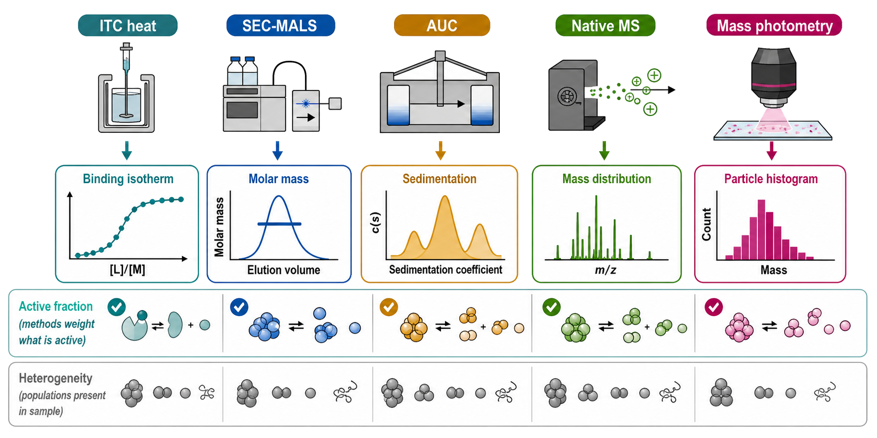
Figure 124.3. Thermodynamic and stoichiometric observables are complementary. “Different methods average heterogeneous RNP states differently. Agreement across heat, mass, hydrodynamics, and activity supports a stoichiometry more strongly than any one fitted n.”
Table 124.3. Stoichiometry and mass methods answer different questions. Match complex heterogeneity to an appropriate method.
| Method | Primary information | Population averaging | Central limitation |
|---|---|---|---|
| ITC | Heat, affinity window, apparent n | Reaction-weighted titration | Active fraction and linked heats |
| SEC-MALS | Molar mass across elution | Coeluting, dilution-shifted population | Exchange during chromatography |
| Sedimentation velocity AUC | Sedimentation and diffusion distributions | Hydrodynamic species distribution | Mass-shape coupling and nonideality |
| Native mass spectrometry | Gas-phase mass and ligand-number distributions | Ionization-selected population | Transfer and gas-phase stability |
| Mass photometry | Single-particle scattering mass near surface | Detected-particle histogram | Surface effects and mass range |
124.4. Real-time and microscale interaction assays: stopped-flow, SPR, BLI, MST, and immobilization effects
Kinetics separates routes that share an affinity
Two interactions can have the same K_D but very different k_on and k_off. A fast-on/fast-off complex and a slow-on/slow-off complex occupy the same equilibrium fraction under a simple model yet respond differently to changing cellular concentrations. For P + R ⇌ PR, pseudo-first-order conditions with one reactant in excess give an observed relaxation rate k_obs = k_on[P] + k_off. Measuring k_obs across several active protein concentrations can estimate the slope and intercept. A competitor-chase experiment can estimate dissociation by suppressing rebinding. Agreement between kinetic k_off/k_on and an independently measured equilibrium K_D is a valuable consistency test, but disagreement can expose multistep binding, inactive fractions, or assay perturbation.
Stopped-flow instruments rapidly mix reactants and record fluorescence, absorbance, or another optical signal beginning after a finite dead time. They are suited to millisecond-to-second association, conformational change, and catalytic events. The observed phase corresponds only to processes that change the selected signal. A rapid binding step followed by fluorescent rearrangement may yield a rate for rearrangement rather than association. Mixing artifacts, photophysics, inner-filter effects, and temperature equilibration need controls. Concentration series and alternative labeling positions help assign phases.
Relaxation methods perturb an equilibrated system by temperature, pressure, or concentration and observe return to equilibrium. Manual mixing covers slower events. Quench-flow converts a transient chemical state into a stable, separable product after defined aging times, making it valuable when no continuous optical signal exists. The time resolution, dead time, quench effectiveness, and recovery efficiency must be characterized for each platform.
Surface plasmon resonance and biolayer interferometry
SPR immobilizes one partner on a sensor surface and detects changes in refractive index near that surface as analyte flows over it. BLI detects changes in optical interference at a biosensor tip during sequential immersion in solutions. Both can generate association and dissociation sensorgrams over multiple analyte concentrations and can estimate kinetic and steady-state parameters. RNA can be immobilized through biotin or another handle, or the protein can be immobilized if RNA remains in solution.
Immobilization changes the geometry. Attachment can block a site, select an orientation, alter folding, or produce a heterogeneous ligand population. High surface density can create avidity, especially for multivalent RBPs and structured RNAs. During association, analyte must be transported from bulk solution to the surface. If transport is slower than molecular binding, the observed rise is mass-transport limited. During dissociation, molecules released near the surface can rebind, making dissociation appear slower. Flow rate, ligand density, analyte concentration, and surface chemistry should be varied to diagnose these regimes.
Reference channels subtract bulk refractive-index changes and nonspecific surface interactions, but reference subtraction cannot repair an active surface that is heterogeneous or overloaded. Blank injections, nonbinding RNA or protein controls, duplicate ligand densities, and regeneration tests are complementary. Regeneration can damage RNA or selectively remove weakly attached material. Single-cycle kinetics avoids regeneration between concentrations but creates its own carryover and model requirements. A clean global 1:1 fit is insufficient if residuals are structured or fitted rates vary with ligand density.
Large RNPs illustrate the mass-transport problem. BLI can detect ribosome-factor interactions and is experimentally convenient, but the large analyte has slow diffusion and may engage immobilized components multivalently. An apparent slow k_off may reflect rebinding. Solution competition, lower loading density, faster mixing, reversed orientation, or an orthogonal solution assay helps distinguish molecular residence time from surface residence.
Microscale thermophoresis and capillary fluorescence methods
MST applies a microscopic temperature gradient and measures fluorescence redistribution and rapid temperature-jump responses in a capillary. Binding can change size, charge, hydration shell, conformation, or dye environment, producing a concentration-dependent signal. One partner is fluorescent and held at nominally constant concentration while the other is titrated. The small volume and broad concentration range are attractive for RNA systems. A standard MST titration is ordinarily interpreted as an equilibrium or apparent-equilibrium binding measurement. It does not inherently supply molecular k_on and k_off values merely because its optical response contains time-resolved phases.
The thermophoretic signal is composite. Fluorescence intensity before heating should be inspected across the titration because ligand-dependent quenching, adsorption, aggregation, or pipetting differences can mimic binding. Capillary scans and multiple excitation powers can reveal some artifacts. Detergent or carrier can suppress sticking but may alter the interaction. As in anisotropy, a fitted curve is interpretable only after demonstrating that the response corresponds to a defined state transition.
Bioanalytical instruments often offer a one-click affinity or kinetic fit. The operator remains responsible for species definitions, active concentrations, mass balance, transport, and response calibration. A physically plausible model should predict how curves change when concentration, orientation, density, time window, or competition is altered.
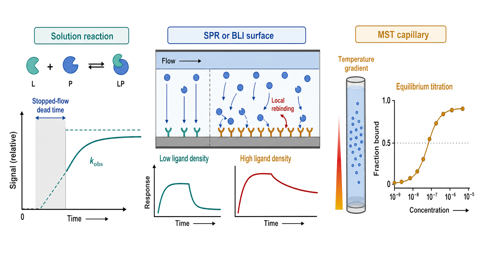
Figure 124.4. Solution kinetics and surface sensorgrams. “Real-time traces contain instrument, transport, response, and molecular timescales. Standard MST titrations report equilibrium-like concentration responses rather than intrinsic k_on and k_off.”
Box 124.1. Diagnose an implausibly slow surface off-rate
- Required questions: Does k_off vary with ligand density? Does faster flow alter association? Does reversed orientation agree? Does a solution competitor chase dissociate faster? Is the analyte multivalent or aggregated? Is reference subtraction adequate? Does regeneration alter the surface? Do residuals support a 1:1 model?
- Misconception prevented: A long dissociation tail always measures a long-lived molecular complex.
124.5. Steady-state, pre-steady-state, single-turnover, and coupled enzymatic assays
Match kinetic regime to the mechanistic question
RNA enzymes include protein enzymes acting on RNA, catalytic RNAs, and RNP catalysts. A minimal scheme might be E + S ⇌ ES → EP ⇌ E + P, but real pathways can include RNA folding, induced fit, chemistry, conformational reset, product release, cofactor exchange, or enzyme inactivation. The purpose of an assay is not to force every system into this minimal scheme. It is to select conditions and observables that distinguish the steps relevant to the question.
Steady-state experiments usually place substrate in excess over active enzyme and measure an initial velocity during repeated turnovers. Under a simple Michaelis-Menten model, v = k_cat[E]_active[S]/(K_M + [S]). k_cat is the limiting turnover rate at saturating substrate for the modeled cycle. K_M is a composite kinetic constant and is not generally a binding K_D. The specificity constant k_cat/K_M describes the low-substrate slope and can reflect productive capture and subsequent commitment steps. Interpretation must name the substrate, ionic conditions, temperature, enzyme active concentration, and observable.
An initial rate is measured before substrate depletion, product accumulation, reverse reaction, enzyme inactivation, or changing assay conditions materially alter the slope. “First five minutes” is not a universal initial-rate window. Progress curves should be inspected and the chosen interval justified across substrate concentrations. A fixed time window can include a lag at low substrate and a curved region at high substrate, creating systematic bias. Replicate rates should come from independently prepared reactions rather than from several readings of one trajectory.
Pre-steady-state experiments observe events before the steady distribution of intermediates is established. With enzyme in excess or comparable to substrate, a rapid product burst followed by a slower linear phase can indicate that chemistry is faster than a later step such as product release, although alternative mechanisms must be considered. Single-turnover conditions often place active enzyme above substrate so that substrate conversion reports steps up to first product formation without requiring enzyme recycling. Multiple-turnover and single-turnover rates therefore answer different questions.
For a ribozyme, endpoint amplitude is as important as rate. A single exponential fraction product = A(1 - e^{-k_obs t}) contains an amplitude A that may reflect the reactive substrate fraction. Normalizing every trace to its own endpoint erases evidence of inactive substrate. Biphasic behavior can represent two substrate populations, sequential steps, heterogeneous metal occupancy, or an inadequately resolved mixing event. Rate constants should not be assigned to molecular steps from curve shape alone.
Substrate series, cofactors, and inhibition
A substrate titration must span the informative region. If all concentrations are far below K_M, the data constrain k_cat/K_M but not k_cat; if all are far above, they constrain k_cat but not K_M. Concentration uncertainty and active fraction should be propagated. RNA substrates can self-associate, fold differently across concentration, bind magnesium, or sequester enzyme nonspecifically. Ionic strength should be controlled when changing a charged substrate or cofactor.
ATP-dependent helicases and remodelers require at least two linked questions: ATP hydrolysis and RNA remodeling. An enzyme can hydrolyze ATP without unwinding the intended duplex, and a fluorescence-unwinding signal can be altered by spontaneous reannealing. Measuring ATPase activity, unwinding amplitude and rate, product trapping, and substrate binding across matched conditions separates chemical consumption from mechanical outcome. Mechanistic ownership of helicase families belongs in their dedicated enzyme chapters; this chapter owns the assay logic.
Inhibitors can compete with substrate, bind an allosteric state, trap a product complex, aggregate, chelate metal, quench signal, or inhibit the coupling enzyme. IC50 depends on assay composition and is not an intrinsic inhibition constant. Time-dependent inhibition requires preincubation and progress-curve analysis. RNA-binding small molecules can change RNA fold rather than directly occupy the enzyme active site. Order-of-addition experiments and orthogonal readouts are therefore mechanistically informative.
Coupled assays report a relay
A coupled assay converts an otherwise difficult primary event into a convenient optical or chemical signal. ATPase activity is often coupled through pyruvate kinase and lactate dehydrogenase to oxidation of NADH, monitored at 340 nm. The observed absorbance change is proportional to ATP turnover only when coupling stoichiometry is known, coupling enzymes and substrates are in excess, the relay reaches its working state rapidly, and none of the primary components perturb the reporters.
Coupling capacity should be challenged by varying coupling-enzyme concentration. If the inferred primary rate changes, the reporter is limiting. A known pulse of product can calibrate response and reveal lag. RNA, protein, salt, small molecules, and test inhibitors can absorb, scatter, quench, inhibit the coupling enzymes, or change background drift. Blanks should omit the primary enzyme, substrate, or cofactor separately rather than rely on one no-enzyme control. Lag phases can arise from slow activation, coupled-reaction buildup, temperature equilibration, or genuine mechanistic transitions.
Discontinuous assays avoid some coupling problems by quenching aliquots and separating substrate and product by gel, chromatography, capillary electrophoresis, mass spectrometry, or sequencing. They introduce quench timing, recovery, separation bias, and endpoint calibration. A denaturing gel can distinguish RNA lengths but may not separate isomers or chemically modified products of equal size. Product identity should be established independently before band intensity is interpreted as chemistry.
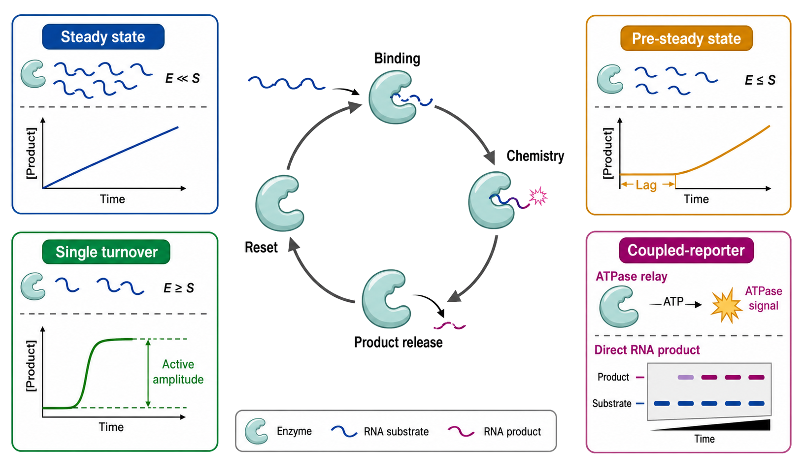
Figure 124.5. Kinetic regimes reveal different portions of an RNA-enzyme cycle. “Repeated turnover averages several steps, whereas transient and single-turnover experiments can expose early events. Coupled assays add a reporter relay that must exceed the primary flux.”
Table 124.4. Enzyme-kinetic regimes and justified conclusions. Keep parameter meaning tied to catalyst/substrate regime and observable.
| Regime | Typical concentration relation | Strong inference | Common overclaim |
|---|---|---|---|
| Steady-state initial rate | Substrate greatly exceeds active enzyme | Cycle-level k_cat and low-substrate slope under model | K_M is substrate K_D |
| Full progress curve | Significant substrate/product change modeled | Depletion, reversibility, inhibition if identifiable | Any curved trace uniquely identifies mechanism |
| Pre-steady state | Early time before steady intermediate distribution | Rapid phases and burst amplitudes | Each exponential is an elementary step |
| Single turnover | Active catalyst exceeds substrate | Steps through first product formation | Rate predicts repeated cellular turnover |
| Coupled continuous assay | Reporter relay in excess | Primary flux if relay is calibrated | Optical signal directly reports RNA chemistry |
124.6. Model fitting, global analysis, parameter identifiability, and uncertainty
Fit the model to the measurement, not only to processed summaries
The statistical model should begin with the chemical reaction network, mass balances, initial conditions, and response function. For a simple equilibrium titration, an analytical equation may be adequate. For multistep kinetics, numerical integration of ordinary differential equations often preserves more information than fitting each trace to one or more exponentials and then fitting the derived rates. Direct fitting of raw progress curves can incorporate substrate depletion, reverse reactions, and shared parameters.
Preprocessing can hide assumptions. Baseline subtraction, normalization, reference-channel subtraction, band segmentation, and removal of an “outlier” all alter the data supplied to the fit. These operations should be defined and, where possible, included as nuisance parameters or sensitivity analyses. Normalizing each binding curve between zero and one discards amplitude information that might reveal inactive material or concentration-dependent response. Fitting log-transformed and untransformed data assigns different error structures.
Residuals should be plotted against concentration and time. Random-looking residuals do not prove the model, but systematic waves, concentration-dependent signs, or differing variance reveal mismatch. Comparing alternative models requires more than the highest R². Additional parameters nearly always improve fit. Information criteria, likelihood-ratio tests for appropriate nested models, held-out predictions, and mechanistically designed perturbations can help, but chemical plausibility and parameter identifiability remain essential.
Global analysis creates leverage and obligations
Global fitting shares selected parameters across datasets. Association traces at several protein concentrations can share k_on and k_off; competition datasets can share tracer affinity; multiple catalytic progress curves can share microscopic rate constants while initial substrate concentrations vary; ITC experiments at different concentrations can share affinity while allowing experiment-specific active fractions or baselines.
The leverage comes from complementary sensitivity. One dataset may constrain a rapid association while another constrains slow dissociation. A solution equilibrium assay can constrain K_D, allowing a surface kinetic fit to test transport or heterogeneity. However, sharing a parameter asserts that temperature, buffer, labeling, active state, and mechanism are common. If data were collected on different days with different preparations, forcing one active fraction or baseline can create false precision. Hierarchical models can distinguish shared biological parameters from experiment-specific nuisance parameters.
Identifiability limits what a curve can say
Structural identifiability asks whether ideal, noise-free observations uniquely determine the parameters of a model. Practical identifiability asks whether the actual concentration range, time resolution, signal-to-noise ratio, and replicate design constrain them. A nonlinear optimizer can return a best-fit value and small local standard error even when a long valley of nearly equivalent parameter combinations exists.
Profile likelihood or explicit confidence-contour calculations vary one parameter and reoptimize the others, revealing asymmetric or unbounded intervals. Bootstrap resampling can represent sampling variability when its resampling unit matches the experimental design. Bayesian posterior distributions can incorporate prior information but should show how strongly priors determine weakly informed parameters. Markov-chain convergence does not make a parameter identifiable. Whatever framework is used, report correlations and boundaries rather than only point estimates.
Experimental design should target sensitivity. To distinguish k_on and k_off, collect time points across the rapid association and slow dissociation phases at several concentrations. To estimate k_cat and k_cat/K_M, sample below and above the transition. To separate active concentration from tight affinity, combine a stoichiometric regime with a lower-concentration equilibrium or competition regime. To test cooperativity, measure stoichiometry and vary concentration over a range that differentiates alternative binding polynomials. Simulation before data collection can expose parameters that the planned experiment cannot recover.
Uncertainty belongs to the biological claim
Technical noise, between-preparation variation, concentration calibration, active fraction, temperature control, and model choice contribute different uncertainties. A confidence interval conditional on one model and fixed concentrations does not include model-form or stock-concentration uncertainty. Report the number and nature of independent replicates, show individual datasets, and distinguish standard deviation, standard error, and parameter confidence intervals.
Parameter units and definitions matter. For a cooperative apparent fit, state whether a reported constant is macroscopic, microscopic, or phenomenological. For surface kinetics, disclose ligand density and transport model. For catalytic fits, state whether enzyme concentration is nominal or active and whether rates are normalized per monomer or complex. Preserve raw or minimally processed data and analysis code where possible. Reproducibility requires the path from recorded signal to reported parameter.
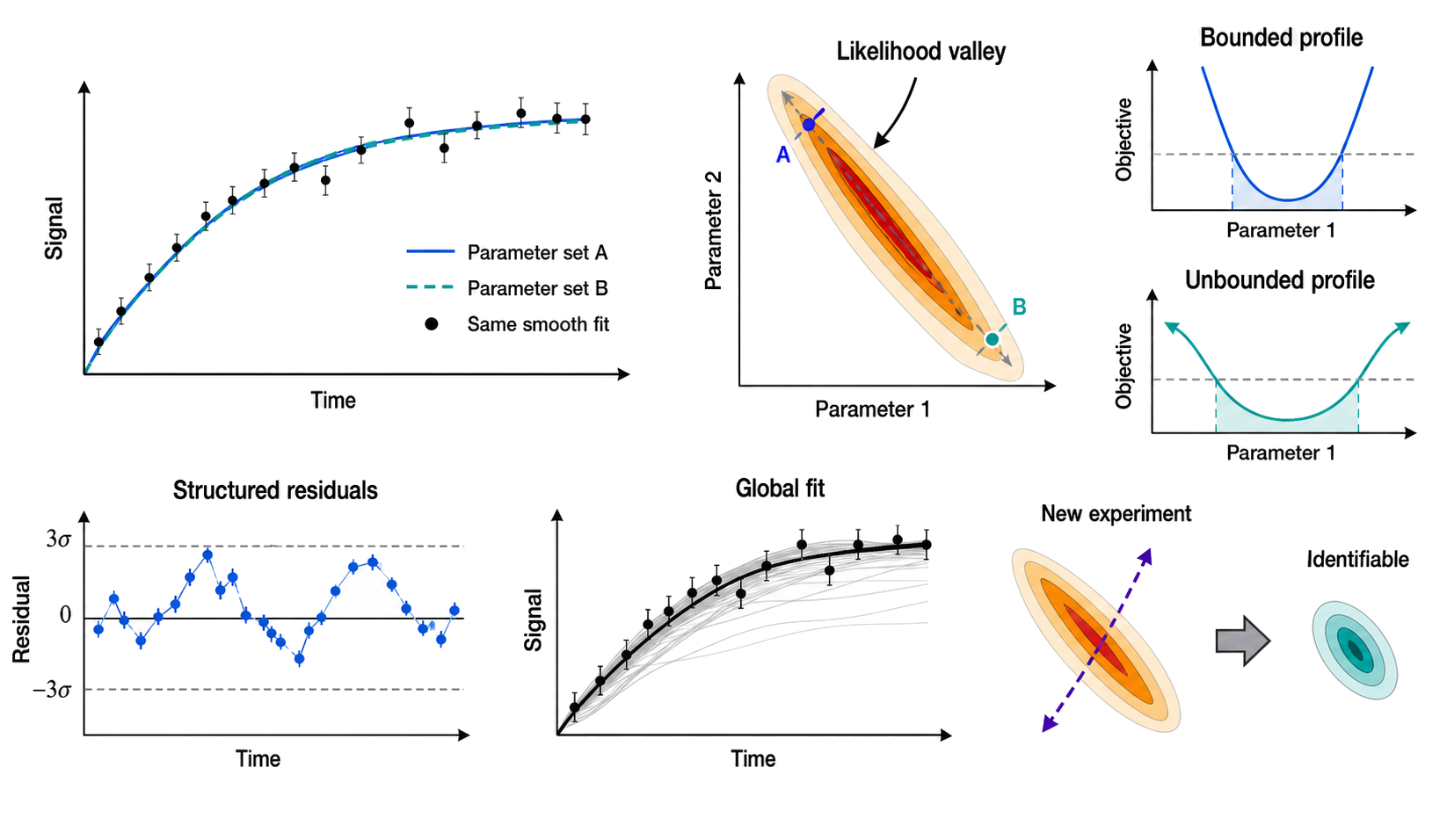
Figure 124.6. A parameter valley can hide behind a smooth fit. “A best-fit point is not enough. Parameter profiles and informative perturbations show whether the experiment constrains a mechanism or only a family of equivalent predictions.”
Table 124.5. Identifiability and uncertainty diagnostics. Pair a fitting symptom with a diagnostic and an experimental response.
| Symptom | Diagnostic | Interpretation | Strong next experiment |
|---|---|---|---|
| Smooth fit but unstable parameter | Profile likelihood or confidence contour | Correlated or weakly constrained parameter | Extend concentration or time range |
| Systematic residual waves | Residuals versus time and concentration | Response or reaction-model mismatch | Add an observable or resolve early time |
| Different fits give different constants | Global fit with justified shared parameters | Separate datasets lack leverage | Collect complementary perturbations |
| Tight confidence interval across technical repeats | Independent preparations and concentration calibration | Shared systematic error omitted | Repeat stock preparation and active titration |
| Complex model always fits better | Penalized comparison and held-out prediction | Extra parameters absorb noise | Design a model-discriminating perturbation |
124.7. Controls, artifacts, orthogonal validation, reporting, and mechanistic handoffs
Controls should target the leading alternative explanation
A good control is defined by the artifact it can reveal. A nonbinding RNA sequence tests sequence-dependent signal but not protein aggregation. A fluorophore-only control tests dye response but not whether labeled RNA retains its native fold. A blank surface tests bulk signal and nonspecific adsorption but not immobilization-induced occlusion. A no-enzyme control tests spontaneous conversion but not whether a coupled reporter is limiting. Each primary claim should list the most plausible nonmechanistic explanation and the control that discriminates it.
Concentration-series controls are unusually powerful. Varying labeled RNA concentration tests ligand depletion. Varying surface density tests rebinding and mass transport. Varying coupling-enzyme concentration tests relay limitation. Varying active enzyme concentration tests whether rates scale as the model predicts. Varying equilibration time tests equilibrium. Varying labeling position tests local perturbation. These controls interrogate the measurement model rather than merely adding negative samples.
Artifacts can be shared across apparently orthogonal assays. Aggregation can create gel shifts, increased anisotropy, surface binding, thermophoretic changes, light-scattering mass, and apparent enzyme inhibition. A fluorophore and a biotin tag are different labels but may both perturb the same RNA terminus. Orthogonality should therefore be defined by physical principle and perturbation, not instrument name.
Orthogonal validation is claim-specific
For an equilibrium affinity, combine a separation method such as EMSA with a homogeneous solution method such as anisotropy or competition, and test concentration and equilibration regimes. For stoichiometry, combine calorimetric equivalence with a mass-sensitive method and an activity measurement. For kinetic rates, compare stopped-flow or chase measurements with equilibrium K_D and use reversed labeling or surface orientation. For catalytic parameters, compare continuous and discontinuous readouts, confirm product identity, and measure active enzyme concentration.
Disagreement is diagnostic. If EMSA gives tighter binding than anisotropy, gel stabilization, dye perturbation, or incomplete equilibration may be involved. If SPR gives a slow k_off but solution chase is fast, rebinding or surface heterogeneity is likely. If ATPase activity increases without RNA unwinding, hydrolysis is uncoupled from remodeling. If ITC stoichiometry is low while native mass shows the expected complex, active fraction or concentration calibration deserves attention.
Reporting checklist
A reproducible report states identities and preparations of all components; sequence and terminal chemistry of RNA; purification and folding history; buffer composition, pH at assay temperature, ions, additives, and temperature; nominal and active concentrations with measurement methods; labeling efficiency and attachment position; order of addition and equilibration; instrument settings and time resolution; raw response and calibration; controls and exclusions; equations or reaction schemes; fixed, shared, and fitted parameters; weighting and error model; replicate structure; residuals and intervals; and availability of data and code. Published surveys show that equilibration and ligand-depletion controls are often missing even when precise affinities are reported.
The strongest conclusion is no broader than the assay. “Puf4 binds this RNA with an apparent K_D under the stated buffer and temperature” is defensible if the equilibrium and concentration assumptions are met. “This RNA is the physiological target” requires cellular occupancy and function from other chapters. “The enzyme cleaves RNA rapidly in a single-turnover assay” does not establish repeated turnover in vivo. “A 2:1 complex forms in solution” does not specify its atomic arrangement.
Mechanistic handoffs
This chapter hands molecular recognition, specificity determinants, and assembly pathways to 56. It hands three-dimensional architectures, conformational ensembles, and structural validation to 59. It hands RNA preparation and general detection calibration that concern abundance rather than molecular activity to 123, and large-scale sequencing assay ownership to the relevant methods chapters. Polymerases, nucleases, helicases, ligases, modification enzymes, ribozymes, ribosomes, spliceosomes, and other RNPs retain their biological and mechanistic narratives in their dedicated chapters. Those chapters should reuse the measurement principles here when evaluating their evidence.
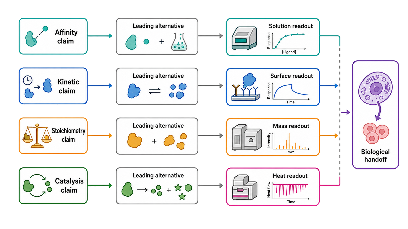
Figure 124.7. Orthogonal validation follows the leading alternative. “Orthogonality means different physical observables and dominant artifacts. The resulting parameter remains conditional on the purified system and hands biological mechanism to the appropriate chapter.”
Table 124.6. Reporting fields for reusable biochemical parameters. Define the minimum context needed to reuse a reported parameter.
| Domain | Required fields | Why it matters |
|---|---|---|
| Material | Sequence, ends, modifications, purification, fold history, active fraction | Defines reacting species and competence |
| Conditions | Buffer, pH, ions, additives, temperature, order of addition | Parameters are condition-dependent |
| Concentrations | Nominal and active values, measurement method, uncertainty | Controls depletion, stoichiometry, and normalization |
| Observable | Label, calibration, instrument settings, time resolution | Maps signal to species |
| Model | Reaction scheme, mass balance, fixed/shared/fitted parameters, error model | Defines parameter meaning |
| Evidence | Independent replicates, residuals, intervals, orthogonal controls | Shows constraint and reproducibility |
| Reuse | Raw data, preprocessing, code, units, censored bounds | Enables reanalysis and synthesis |
Experimental Foundations and Evidence
Quantitative biochemical evidence is strongest when several levels agree. Material characterization establishes what entered the assay. A calibrated observable reports a physical transition. Concentration and time perturbations test the mathematical model. Orthogonal measurements challenge assay-specific artifacts. Structural or cellular experiments then connect the in vitro state to biological mechanism. Failure at one level does not erase the others, but it narrows the claim.
Historical binding and kinetic equations remain foundational, yet modern instruments do not remove classical constraints. High sensitivity can make adsorption and impurities more important. Automated fitting can conceal nonidentifiability. High throughput can multiply systematic bias. The evidence standard should therefore scale with the consequence of the parameter: a mechanistic rate assignment needs more support than a screening rank order, and a therapeutic selectivity claim needs matrix, reproducibility, and off-target controls beyond a purified binary interaction.
Biological Contexts Across Organisms, Cell Types, and Perturbations
Purified assays deliberately isolate reactions, but the chosen conditions should reflect the biological question. Bacterial RBPs may encounter high RNA and magnesium concentrations in compact cytoplasm; nuclear RNP assembly may depend on multivalent partners and cotranscriptional order; viral RNPs may form on membrane-associated templates; therapeutic oligonucleotides may bind proteins at concentrations and ionic conditions unlike a standard buffer. These contexts do not invalidate reductionist measurements. They define which components and perturbations should be added next.
Comparative claims require matched competence. An ortholog that expresses poorly or aggregates cannot be declared to have weaker RNA affinity solely from nominal concentration. A disease variant that changes protein stability may reduce active fraction without changing the microscopic affinity of competent molecules. A modified RNA may change absorbance, fold, label response, or nuclease stability as well as molecular recognition. Controls should separate amount, competence, and intrinsic parameter.
Technology, Computational, Clinical, and Engineering Links
Quantitative binding and catalytic data support RNA sensor design, aptamer selection, guide-RNA optimization, enzyme engineering, inhibitor discovery, and therapeutic quality control. Engineering needs parameters measured in the intended operating range. An aptamer selected for endpoint occupancy may switch too slowly for a dynamic sensor. A guide RNP with tight equilibrium binding may release product too slowly for turnover. A small molecule with attractive IC50 can fail because the apparent inhibition arose from aggregation or reporter interference.
Computational models benefit from full curves and uncertainty rather than isolated best-fit constants. Training or benchmarking on unqualified affinity tables can merge values measured with different active fractions, buffers, temperatures, models, and assay geometries. Machine-learning predictions should be compared with prospectively designed measurements that include failed or censored experiments and distinguish bounds from identified values.
Recent Consensus
Current quantitative-biochemistry practice converges on several principles. The equilibrium state must be demonstrated rather than assumed. Free and total concentration regimes must be distinguished, especially for tight binding. Active concentration and sample competence are first-order experimental variables. Multiple observables or perturbations are needed before a fitted kinetic phase is assigned to a molecular step. Surface methods require explicit evaluation of immobilization, mass transport, rebinding, and nonspecific binding. Michaelis-Menten parameters are regime-dependent summaries and K_M is not generally K_D. Global fitting is most valuable when shared parameters are justified and confidence contours or equivalent diagnostics show that those parameters are constrained.
Open Questions, Controversies, Deprecated Models, and Common Misconceptions
Open questions:
- How can active fractions of heterogeneous, multicomponent RNPs be measured without assuming the same stoichiometry or mechanism that the experiment seeks to test?
- Which minimal sets of orthogonal measurements best identify multistep RNA recognition mechanisms while preserving scarce material?
- How should model uncertainty and preparation-to-preparation variability be standardized across public databases of RNA affinity and enzyme kinetics?
- When do in vitro solution parameters remain predictive in condensates, membranes, crowded compartments, or cotranscriptional assembly pathways?
Controversies:
- Complex binding curves can often be fit by several cooperative, conformational-selection, induced-fit, or heterogeneous-population models. A statistically preferred fit rarely settles mechanism without an independent perturbation that distinguishes states.
- Some workflows report highly precise surface-derived residence times for multivalent RNPs. The degree to which these represent molecular dissociation rather than surface rebinding remains system- and design-dependent.
Deprecated or weakened claims:
- A high
R²and visually smooth curve are no longer adequate evidence that a mechanistic model or its parameter errors are reliable. - Fixing a nonintegral ITC stoichiometry to one without independent concentration or activity evidence is not a neutral correction.
Common misconceptions:
- “The concentration measured by absorbance is the active concentration.” Bulk concentration counts signal-producing material; competence must be measured for the stated reaction.
- “The protein concentration at half-maximal binding always equals
K_D.” That equality requires an appropriate simple model, equilibrium, and a concentration regime without important ligand depletion. - “A Hill coefficient of two proves two cooperative sites.” A Hill slope is phenomenological and can reflect multiple sites, depletion, heterogeneity, or signal distortion.
- “Label-free means perturbation-free.” ITC avoids a reporter label, but buffer mismatch and linked heats matter; SPR and BLI avoid analyte labels but immobilize one partner.
- “
K_Mmeasures substrate binding affinity.”K_Mis a kinetic composite except under restricted mechanisms and rate relationships. - “A fitted microscopic rate is identified because software returns a standard error.” Local optimizer errors can remain small along a broad correlated parameter valley.
- “Two instruments provide orthogonal validation.” Orthogonality depends on independent physical observables and artifacts, not brand or platform count.